Formatting data
- Parts of the main Calc window
- Starting new spreadsheets
- Opening existing spreadsheets
- Saving spreadsheets
- Navigating within spreadsheets
- Selecting items in a sheet or a spreadsheet
- Working with spreadsheets
- Viewing Calc
- Entering data using the keyboard
- Speeding up data entry
- Editing data
- Formatting data
- Autoformatting cells and sheets
- Formatting spreadsheets using themes
- Hiding and showing data
- Sorting records
- Printing from Calc
The data in Calc can be formatting in several ways. It can either be edited as part of a cell style so that it is automatically applied, or it can be applied manually to the cell. Some manual formatting can be applied using toolbar icons. For more control and extra options, select the appropriate cell or cells, right-click on it, and select Format Cells. All of the format options are discussed below.
| All the settings discussed in this section can also be set as a part of the style using the Styles and Formatting window. For more information see Chapter 4 of the Calc Guide |
Formatting multiple lines of text
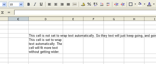
Multiple lines of text can be entered into a single cell using automatic wrapping or manual line breaks. Each method is useful for different situations.
Using automatic wrapping
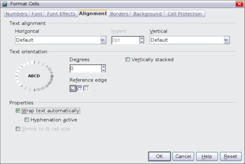
To set text to wrap at the end of the cell, right-click on the cell and select Format Cells (or choose Format > Cells from the menu bar, or press Ctrl+1). On the Alignment tab, under Properties, select Wrap text automatically.
Using manual line breaks
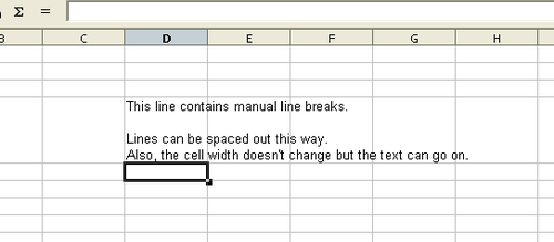
To insert a manual line break while typing in a cell, press Ctrl+Enter. This method does not work with the cursor in the input line. When editing text, first double-click the cell, then single-click at the position where you want the line break.
When a manual line break is entered, the cell width does not change. The figure below shows the results of using two manual line breaks after the first line of text.
Shrinking text to fit the cell
The font size of the data in a cell can automatically adjust to fit in a cell. To do this, select the Shrink to fit cell option in the Format Cells dialog. The figure below shows the results.
Formatting numbers
Several number formats can be applied to cells by using icons on the Formatting toolbar. Select the cell, then click the relevant icon.
![]()
Number format icons. Left to right: currency, percentage, date, exponential, standard, add decimal place, delete decimal place.
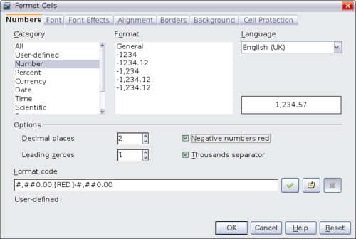
For more control or to select other number formats, use the Numbers tab.
- Apply any of the data types in the Category list to the data.
- Control the number of decimal places and leading zeros.
- Enter a custom format code.
The Language setting controls the local settings for the different formats such as the date order and the currency marker.
Formatting the font
To quickly choose the font used in a cell, select the cell, then click the arrow next to the Font Name box on the Formatting toolbar and choose a font from the list.
| To choose whether to show the font names in their font or in plain text, go to Tools > Options > OpenOffice.org > View and select or deselect the Show preview of fonts option in the Font Lists section. For more information, see Chapter 14: Setting up and Customizing Calc |
To choose the size of the font, click the arrow next to the Font Size box on the Formatting toolbar. For other formatting, you can use the Bold, Italic, or Underline icons.
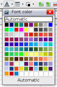
To choose a font color, click the arrow next to the Font Color icon to display a color palette. Click on the required color.
(To define custom colors, use Tools > Options > OpenOffice.org > Colors. See Chapter 14 of the Calc Guide for more information.)
To specify the language of the cell (useful because it allows different languages to exist in the same document and be spell checked correctly), use the Font tab of the Format Cells dialog. Use the Font Effects tab to set other font characteristics. See Chapter 4 of the Calc Guide for more information.
Formatting the cell borders
To quickly choose a line style and color for the borders of a cell, click the small arrows next to the Line Style and Line Color icons on the Formatting toolbar. In each case, a palette of choices is displayed.
For more control, including the spacing between the cell borders and the text, use the Borders tab of the Format Cells dialog. There you can also define a shadow. See Chapter 4 of the Calc Guidefor details.
Formatting the cell background
To quickly choose a background color for a cell, click the small arrow next to the Background Color icon on the Formatting toolbar. A palette of color choices, similar to the Font Color palette, is displayed.
(To define custom colors, use Tools > Options > OpenOffice.org > Colors. See Chapter 14 of the Calc Guide for more information.)
You can also use the Background tab of the Format Cells dialog. See Chapter 4 of the Calc Guide for details.
| Content on this page is licensed under the Creative Common Attribution 3.0 license (CC-BY). |
