Creating formulas
Introduction
By convention, only three kinds of data can be entered in a cell. Text, Numbers, and Formulas. You can enter formulas in two ways, either in the cell itself, or at the input line. Either way you will need to start it with one of the following symbols: "=", "+" or "-". Starting with anything else will cause the formula to be treated as if it were text.
公式運算子
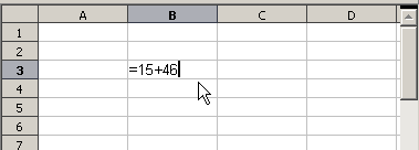
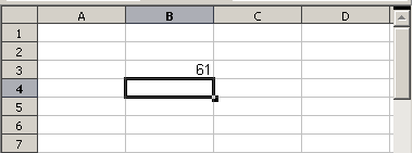
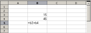
每個單元格在工作表可以作為一個資料持有人或一個地方的資料計算。在鍵入單元格中輸入數據,並移動到下一個單元格或按下鍵。以公式等號表明,該單元格將用於計算。像這樣的數學計算15 + 46,可實現如下所示。
| Simple Calculation in 1 Cell | Calculation by Reference |
|
|
|
|
|
A simple calculation.
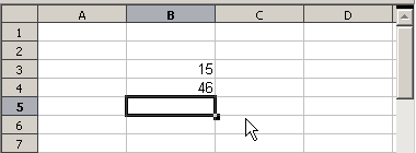
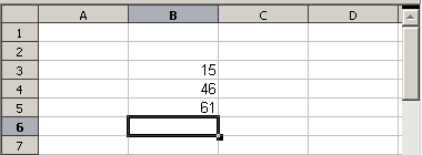
While the calculation on the left was accomplished in only one cell, the real power is shown on the right where the data is placed in cells and the calculation is performed using references back to the cells. In this case, cells B3 and B4 were the data holders with B5 the cell where the calculation was performed. Note that the formula was shown as =B3 + B4. The plus sign indicates that the contents of cells B3 and B4 are to be added together and then have the result in the cell holding the formula. All formulas build upon this concept. Other ways of entering formulas are shown in Table 1.
These cell references allow formulas to use data from anywhere in the worksheet being worked on or from any other worksheet in the workbook that is opened. If the data needed was on different worksheets they would be referenced by referring to the worksheet, for example =SUM(Sheet2.B12+Sheet3.A11).
Table 1: Common ways to enter formulas.
| Formula | Description |
|---|---|
| =A1+10 | 單元內容顯示A1加10。 |
| =A1*16% | 單元內容顯示A1x16%. |
| =A1 * A2 | 單元內容顯示A1xA2 |
| =ROUND(A1;1) | 單元內容顯示A1四捨五入到小數點下一位 |
| =EFFECTIVE(5%;12) | 計算實際利率為每年5%的名義利率與並依12年支付 |
| =B8-SUM(B10:B14) | 計算B8減去B10到B14的總合 |
| =SUM(B8;SUM(B10:B14)) | 先計算B10到B14的總合,再計算B8到SUM(B10:B14)的總合. |
| =SUM(B1:B65536) | 所有數字總合在B顯示 |
| =AVERAGE(BloodSugar) | 計算BloodSugar的平均數 |
| =IF(C31>140; "HIGH"; "OK") | 結果顯示有條件分析資料來源有兩個。 如果C31=144,那麼HIGH會顯示,否則OK顯示。 |
Functions can be identified in Table 1 with a word, for example ROUND, followed by parentheses enclosing references or numbers.
It is also possible to establish ranges for inclusion by naming them using Insert > Names, for example BloodSugar representing a range such as B3:B10. Logical functions can also be performed as represented by the IF statement which results in a conditional response based upon the data in the identified cell.
運算類型
You can use the following operators in OpenOffice.org Calc: arithmetic, comparative, text, and reference.
算術運算
加法,減法,乘法和除法運算符的數值結果。數字的負號,例如-37。 這個例子說明了如何輸入數字正在乘以本身一定數量的日子,例如2的三次方 = 2 * 2 * 2。
Table 2: Arithmetical operators
| Operator | Name | Example |
| + (Plus) | 加法 | =1+1 |
| - (Minus) | 減法 | =2-1 |
| - (Minus) | 負號 | -5 |
| * (asterisk) | 乘法 | =2*2 |
| / (Slash) | 除法 | =10/5 |
| % (Percent) | 百分比 | 15% |
| ^ (Caret) | 次方 | 2^3 |
比較運算
在比較公式中,使用IF函數,並得到一個真或假的答案,例如,=IF(B6>G12; 127; 0),簡單來說,就是如果內容單元格B6超過G12,就得到127,否則得到0。
輸入一個公式,回答TRUE或FALSE,如=B6>B12.。如果答案正確,答案則返回true,否則返回FALSE。
Table 3: Comparative operators
| Operator | Name | Example |
| = (equal sign) | 等於 | A1=B1 |
| > (Greater than) | 大於 | A1>B1 |
| < (Less than) | 小於 | A1<B1 |
| >= (Greater than or equal to) | 大於或等於 | A1>=B1 |
| <= (Less than or equal to) | 小於或等於 | A1<=B1 |
| <> (Inequality) | 不等式 | A1<>B1 |
文字運算
這是常見於電子表格中的文字運算。為了提供變化,以及如何在這種類型的資料顯示,文字可連接在來自不同地方的電子表格。下面就是一個例子。
Text Concatenation.
In this example, specific pieces of the text were found in three different cells. To join these segments together, the formula also adds required spaces and punctuation housed within quotation marks resulting in a formula of =B6 & " " & C6 & ", " D6. The result is the concatenation into a correctly formatted date for this locale.
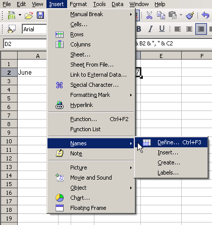
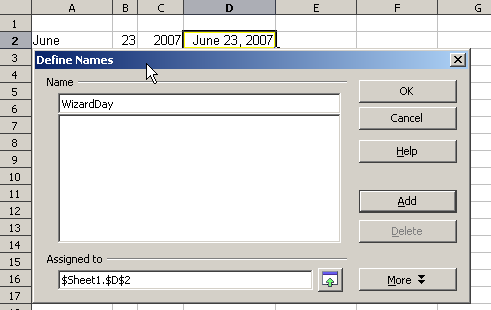
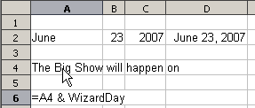
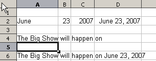
Taking this example further, the result cell is defined as a name, then text concatenation is performed using this defined name.
定義工作表名稱.
參考運算
最簡單的就是引用一個儲存格。但是,參考也可以參考矩形或長方體範圍或參考是一個列表的引用。要建立這樣的引用,你需要引用運算符。
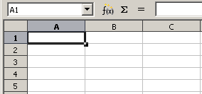
儲存格的命名,以從儲存格的欄(字元)和列(編號)命名。 在電子表格讀取從左到右,左上角單元格A1。下圖顯示了這些儲存格A1。
範圍運算
The range operator is written as colon. An expression using the range operator has the syntax
reference left : reference right
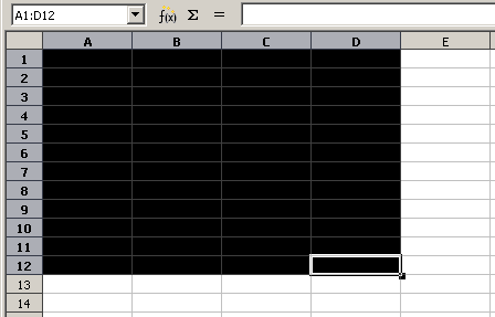
範圍符號為一個參考到最小的範圍,包括儲存格引用的左參考和引用的儲存格的權利。
The picture should be exchanged with one using the new transparent highlighting for selections. Regina 18:33, 19 September 2009 (UTC)
In the upper left corner of the figure above, the reference A1:D12 is shown, corresponding to the cells included in the drag operation with the mouse to highlight the range.
The following is about selecting and naming cells and should be moved somewhere else or be dropped.Regina 18:33, 19 September 2009 (UTC)
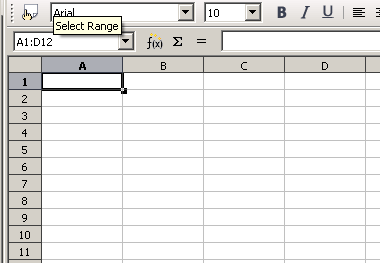
[start to move or drop] This same range could also be created <--wrong term! by entering in the Name Box directly as shown below. After pressing Enter, the same range is selected.
A reference operator <--wrong term! can also be created by defining a named area by selecting the menu item Insert > Names > Define, pressing Ctrl+F3, or clicking the icon, if it shows on your toolbar.
[end to move or drop]
Examples
| A2:B4 | 參考一矩形範圍6單元,2 × 3列寬行高。 |
| (A2:B4):C9 | 參考範圍的矩形由左上角儲存格A2至c9右下角。因此,範圍包含24個儲存格,3× 8。 |
| Sheet1.A3:Sheet3.D4 | 參考範圍長方體共24個儲存格,4× 2 × 3 |
When you enter B4:A2 or A4:B2 directly, then OOo will turn it to A2:B4. So the left top cell of the range is left of the colon and the bottom right cell is right of the colon. But if you name the cell B4 for example with '_start' and A2 with '_end', you can use _start:_end without any error.
OOo can not reference a whole column of unspecified length via A:A or a whole row via 1:1 yet as you might know from other spreadsheet programs, see Issue 20495 .
參考連結運算
連接運算符被寫為波形。表達式為使用連接運算符的語法
reference left ~ reference right
The result of such an expression is a reference list, which is an ordered list of references. Some functions can take a reference list as argument, SUM, MAX or INDEX for example.
The reference concatenation is sometimes called 'union'. But it is no set union. COUNT(A1:C3~B2:D2) returns 12 (=9+3), whereas looking at it as set of cells, it has only 10 cells.
Notice that SUM(A1:C3;B2:D2) is different from SUM( A1:C3~B2:D2) although they give the same result. The first is a function call with 2 parameters, each of them is reference to a range. The second is a function call with 1 parameter, which is a reference list.
交集運算
交集運算符寫成感嘆號。
reference left ! reference right
If the references refer to single ranges, the result is a reference to a single range, containing all cells, which are both in the left reference and in the right reference.
If the references are reference lists, than each list item from the left is intersected with each one from the right and these results are concatenated to a reference list. The order is, to first intersect the first item from the left with all items from the right, then intersect the second item from the left with all items from the right, and so on.
Examples
| A2:B4 ! B3:D6 | 這個結果的範圍是B3:B4,因為儲存格A2:B4和B3:D4的內部 |
| (A2:B4~B1:C2) ! (B2:C6~C1:D3) | 首先可以見成 A2:B4!B2:C6, A2:B4!C1:D3, B1:C2!B2:C6 and B1:C2!C1:D3來計算. 結果是在 B2:B4, 空的, B2:C2, 和C1:C2. 然而這些結果是有交集的,並在空的部分. 所以最後的結果必須參考 B2:B4 ~ B2:C2 ~ C1:C2. |
You can use the intersection operator to refer a cell in a cross tabulation in an good understandable way. If you have columns labeled 'Temperature' and 'Precipitation' and the rows labeled 'January', 'February', 'March',… then the expression
'February' ! !Temperature'
will reference to the cell containing the temperature in February.
The intersection operator ! should have a higher precedence than the concatenation operator ~, but in OOo3.1 it is wrong implemented. Therefore you should not rely on precedence, but always put the part which to be first calculated in parentheses.
計算的順序
Order of calculation refers to the sequence that numerical operations are performed. Division and multiplication are performed before addition or subtraction. There is a common tendency to expect calculations to be made from left to right as the equation would be read in English. Calc evaluates the entire formula, then based upon programming precedence breaks the formula down executing multiplication and division operations before other operations. Due to this fact when creating formulas you should test your formula to make sure that the correct result is being obtained. An example of order of calculation in operation follows.
Table 4 – Order of Calculation
| Left To Right Calculation | Ordered Calculation |
| 1+3*2+3 = 11 | =1+3*2+3 result 10 |
| 1+3=4, then 4 X 2 = 8, then 8 + 3 = 11 | 3*2=6, then 1 + 6 + 3 = 10 |
| Another possible intention could be: | The program resolves the multiplication of 3 X 2 before dealing with the numbers being added. |
| 1+3*2+3 = 20 |
If you intend for the result to be either of the two possible solutions on the left, the way to achieve these results would be to order the formula as:
| ((1+3) * 2)+3 = 11 | (1+3) * (2+3) = 20 |
| Consider using parentheses grouping operations to avoid obtaining incorrect calculations, e.g. = B4+G12*C4/M12 becoming =((B4+G12)*C4)/M12. |
Calculations linking sheets
Another powerful feature of Calc is the ability to link data through several worksheets. The naming of worksheets can be helpful to identify where specific data may be found. A name such a Payroll or Boise Sales is much more meaningful than Sheet1. The function named SHEET() returns the sheet number in the collection of spreadsheets. With this function, if you are currently on the third sheet counting from the left along the worksheet tabs, the number 3 is returned. If you drag the worksheets around to different locations among the tabs, the number will return the number referring to the current position of this worksheet.
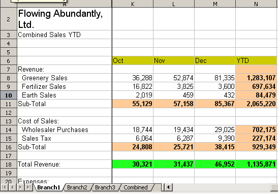
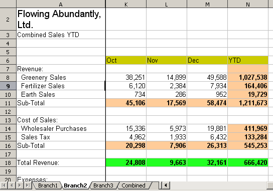
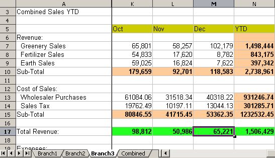
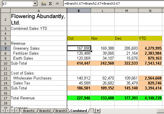
An example of calculations obtaining data from other work can be seen in a business setting where a business combines its branch operations into a single worksheet.
|
Sheet containing data for Branch 1. |
|
Sheet containing data for Branch 2. |
|
Sheet containing data for Branch 3. |
|
Sheet containing combined data for all branches. |
Combining data from several sheets into a single sheet.
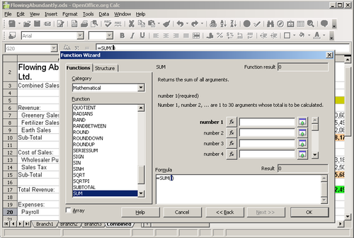
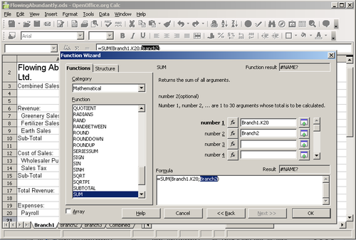
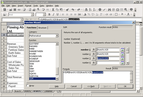
To accomplish the links, it can be easier if the Function Wizard is used.
- Open the Function Wizard by clicking the f(x) button on the toolbar, or by selecting Insert > Function, or by pressing Ctrl+F2.
- Select a category of functions to shorten the list, then scroll down through the named functions and select the required one. When you select a function, its description appears on the right-hand side of the dialog. Double-click on the required function.
- The wizard now displays an area to the right where you can enter data manually in text boxes or click the Shrink button [[Image:]] to shrink the wizard so you can select the cells from the worksheet.
- To select cells, either click directly upon the needed cell or hold down the left mouse button and drag to select the needed area.
- When the area has been selected, click the Shrink button again to return to the wizard.
- If multiple ranges are needed, then select the next text box below the first and perform the same task for the next range. The wizard will accept in the Sum function up to 30 such ranges.
The following figures show how to create the combined sheet shown in the example above.
Strategies for creating formulas
There are several broad approaches when making a decision to create a formula. In deciding on an approach, consider how many other people will need to use the worksheets, the life of the worksheets, and the variations that could be encountered from use.
Enter a unique formula in each cell
The first and most basic strategy is to view whatever formulas are needed as simple and with a limited use life. The strategy is then to place a unique formula in each appropriate cell.
Break formulas into parts and combine the parts
The second strategy is similar, but instead you break down longer formulas into smaller parts and then combine the parts into the whole.
Editor's note: This needs some explanation, but it is NOT about the "formula editor" (Math).
Use the Basic editor to create functions
A third strategy is to use the Basic editor and create your own functions. This approach would be used where the result would greatly simplify the use of the spreadsheet by the end user and keep the formulas simple with a better chance of avoiding errors. This approach also can make the maintenance easier by having corrections or updates kept in one central location. The use of macros is described in Chapter 12 of this book.
| Content on this page is licensed under the Creative Common Attribution 3.0 license (CC-BY). |


