Creating formulas
Creating formulas
You can enter formulas in two ways, either directly into the cell itself, or at the input line. Either way, you need to start a formula with one of the following symbols: =, + or -. Starting with anything else causes the formula to be treated as if it were text.
Operators in formulas
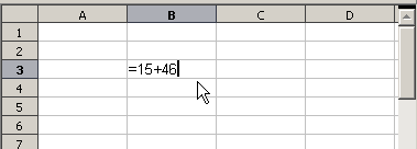
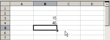
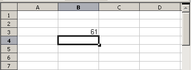
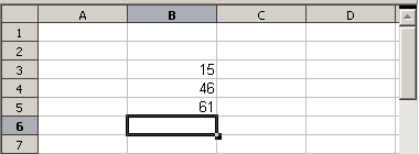
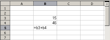
Each cell on the worksheet can be used as a data holder or a place for data calculations. Entering data is accomplished simply by typing in the cell and moving to the next cell or pressing Enter. With formulas, the equals sign indicates that the cell will be used for a calculation. A mathematical calculation like 15 + 46 can be accomplished as shown below.
| Simple Calculation in 1 Cell | Calculation by Reference |
|
|
|
|
|
Above: A simple calculation.
While the calculation on the left was accomplished in only one cell, the real power is shown on the right where the data is placed in cells and the calculation is performed using references back to the cells. In this case, cells B3 and B4 were the data holders with B5 the cell where the calculation was performed. Note that the formula was shown as =B3 + B4. The plus sign indicates that the contents of cells B3 and B4 are to be added together and then have the result in the cell holding the formula. All formulas build upon this concept. Other ways of entering formulas are shown in Table 1.
These cell references allow formulas to use data from anywhere in the worksheet being worked on or from any other worksheet in the workbook that is opened. If the data needed was on different worksheets they would be referenced by referring to the worksheet, for example =SUM(Sheet2.B12+Sheet3.A11).
Table 1: Common ways to enter formulas.
| Formula | Description |
|---|---|
| =A1+10 | Displays the contents of cell A1 plus 10. |
| =A1*16% | Displays 16% of the contents of A1. |
| =A1 * A2 | Displays the result of the multiplication of A1 and A2. |
| =ROUND(A1;1) | Displays the contents of cell A1 rounded to one decimal place. |
| =EFFECTIVE(5%;12) | Calculates the effective interest for 5% annual nominal interest with 12 payments a year. |
| =B8-SUM(B10:B14) | Calculates B8 minus the sum of the cells B10 to B14. |
| =SUM(B8;SUM(B10:B14)) | Calculates the sum of cells B10 to B14 and adds the value to B8. |
| =SUM(B1:B65536) | Sums all numbers in column B. |
| =AVERAGE(BloodSugar) | Displays the average of a named range defined under the name BloodSugar. |
| =IF(C31>140; "HIGH"; "OK") | Displays the results of a conditional analysis of data from two sources. If C31 = 144, then HIGH is displayed, otherwise OK is displayed. |
Functions can be identified in Table 1 with a word, for example ROUND, followed by parentheses enclosing references or numbers.
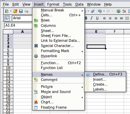
It is also possible to establish ranges for inclusion by naming them using Insert > Names, for example BloodSugar representing a range such as B3:B10. Logical functions can also be performed as represented by the IF statement which results in a conditional response based upon the data in the identified cell.
=IF(A2>=0;"Positive";"Negative")
A value of 3 in cell A2 would return the result Positive, -9 the result Negative.
Operator types
You can use the following operators in OpenOffice.org Calc: arithmetic, comparative, text, and reference.
Arithmetic operators
The addition, subtraction, multiplication and division operators return numerical results. The Negation and Percent operators identify a characteristic of the number found in the cell, for example -37. The example for Exponentiation illustrates how to enter a number that is being multiplied by itself a certain number of times, for example 23 = 2*2*2.
Table 2: Arithmetical operators
| Operator | Name | Example |
| + (Plus) | Addition | =1+1 |
| - (Minus) | Subtraction | =2-1 |
| - (Minus) | Negation | -5 |
| * (asterisk) | Multiplication | =2*2 |
| / (Slash) | Division | =10/5 |
| % (Percent) | Percent | 15% |
| ^ (Caret) | Exponentiation | 2^3 |
Comparative operators
Comparative operators are found in formulas that use the IF function and return either a true or false answer; for example, =IF(B6>G12; 127; 0) which, loosely translated, means if the contents of cell B6 are greater than the contents of cell G12, then return the number 127, otherwise return the number 0.
A direct answer of TRUE or FALSE can be obtained by entering a formula such as =B6>B12. If the numbers found in the referenced cells are accurately represented, the answer TRUE is returned, otherwise FALSE is returned.
Table 3: Comparative operators
| Operator | Name | Example |
| = (equal sign) | Equal | A1=B1 |
| > (Greater than) | Greater than | A1>B1 |
| < (Less than) | Less than | A1<B1 |
| >= (Greater than or equal to) | Greater than or equal to | A1>=B1 |
| <= (Less than or equal to) | Less than or equal to | A1<=B1 |
| <> (Inequality) | Inequality | A1<>B1 |
If cell A1 contains the numerical value 4 and cell B1 the numerical value 5, the above examples would yield results of FALSE, FALSE, TRUE, FALSE, TRUE, and TRUE.
Text operators
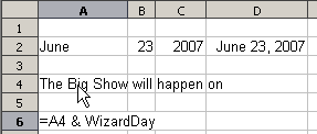
It is common for users to place text in spreadsheets. To provide for variability in what and how this type of data is displayed, text can be joined together in pieces coming from different places on the spreadsheet. Below is an example.
Text Concatenation.
In this example, specific pieces of the text were found in three different cells. To join these segments together, the formula also adds required spaces and punctuation housed within quotation marks resulting in a formula of =B6 & " " & C6 & ", " D6. The result is the concatenation into a date formatted in a particular sequence.
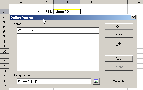
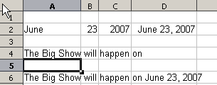
Taking this example further, the result cell is defined as a name, then text concatenation is performed using this defined name. Calc has a CONCATENATE function which performs the same operation.
Defining Names on a worksheet.
Reference operators
In its simplest form a reference refers to a single cell, but references can also refer to a rectangle or cuboid range or a reference in a list of references. To build such references you need reference operators.
An individual cell is identified by the column identifier (letter) located along the upper edge of the spreadsheet and a row identifier (number) found along the side of the spreadsheet. On spreadsheets read from left to right, the upper left cell is A1.
Range operator
The range operator is written as colon. An expression using the range operator has the following syntax:
reference left : reference right
The range operator builds a reference to the smallest range including both the cells referenced with the left reference and the cells referenced with the right reference.
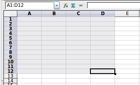
In the upper left corner of the figure above, the reference A1:D12 is shown, corresponding to the cells included in the drag operation with the mouse to highlight the range.
Examples
| A2:B4 | Reference to a rectangle range with 6 cells, 2 column width × 3 row height. When you click on the reference in the formula in the input line, a border indicates the rectangle. |
| (A2:B4):C9 | Reference to a rectangle range with cell A2 top left and cell C9 bottom right. So the range contains 24 cells, 3 column width × 8 row height. |
| Sheet1.A3:Sheet3.D4 | Reference to a cuboid range with 24 cells, 4 column width × 2 row height × 3 sheets depth. |
When you enter B4:A2 or A4:B2 directly, then Calc will turn it to A2:B4. So the left top cell of the range is left of the colon and the bottom right cell is right of the colon. But if you name the cell B4 for example with '_start' and A2 with '_end', you can use _start:_end without any error.
Calc can not reference a whole column of unspecified length via A:A or a whole row via 1:1 yet as you might know from other spreadsheet programs, see Issue 20495 .
Reference Concatenation Operator
The concatenation operator is written as tilde. An expression using the concatenation operator has the following syntax
reference left ~ reference right
The result of such an expression is a reference list, which is an ordered list of references. Some functions can take a reference list as argument, SUM, MAX or INDEX for example.
The reference concatenation is sometimes called 'union'. But it is not the union of two sets, 'reference left' and 'reference right' as normally understood in set theory. COUNT(A1:C3~B2:D2) returns 12 (=9+3), but it has only 10 cells when considered as the union of the two sets of cells.
Notice that SUM(A1:C3;B2:D2) is different from SUM( A1:C3~B2:D2) although they give the same result. The first is a function call with 2 parameters, each of them a reference to a range. The second is a function call with 1 parameter, which is a reference list.
Intersection Operator
The intersection operator is written as exclamation mark. An expression using the intersection operator has the following syntax
reference left ! reference right
If the references refer to single ranges, the result is a reference to a single range, containing all cells, which are both in the left reference and in the right reference.
If the references are reference lists, than each list item from the left is intersected with each one from the right and these results are concatenated to a reference list. The order is, to first intersect the first item from the left with all items from the right, then intersect the second item from the left with all items from the right, and so on.
Examples
| A2:B4 ! B3:D6 | This results a reference to the range B3:B4, because these cells are inside A2:B4 and inside B3:D4. |
| (A2:B4~B1:C2) ! (B2:C6~C1:D3) | First the intersections A2:B4!B2:C6, A2:B4!C1:D3, B1:C2!B2:C6 and B1:C2!C1:D3 are calculated. This results in B2:B4, empty, B2:C2, and C1:C2. Then these results are concatenated, dropping empty parts. So the final result is the reference list B2:B4 ~ B2:C2 ~ C1:C2. |
You can use the intersection operator to refer a cell in a cross tabulation in an understandable way. If you have columns labeled 'Temperature' and 'Precipitation' and the rows labeled 'January', 'February', 'March',… then the expression
'February' ! !Temperature'
will reference to the cell containing the temperature in February.
The intersection operator (!) should have a higher precedence than the concatenation operator (~), but do not rely on the precedence.
Relative and absolute references
References are the way that we refer to the location of a particular cell in Calc and can be either relative (to the current cell) or absolute (a fixed amount).
Relative referencing
An example of a relative reference will illustrate the difference between a relative reference and absolute reference using the spreadsheet shown below.
- Type the numbers 4 and 11 into cells C3 and C4 respectively of that spreadsheet.
- Copy the formula in cell B5 to cell C5. You can do this by using a simple copy and paste or click and drag B5 to C5 as shown below. The formula in B5 calculates the sum of values in the two cells B3 and B4.
- Click in cell C5. The formula bar shows =C3+C4 rather than =B3+B4 and the value in C5 is 15, the sum of 4 and 11 which are the values in C3 and C4.
In cell B5 the references to cells B3 and B4 are relative references. This means that Calc interprets the formula in B5 and applies it to the cells in the B column and puts the result in the in the cell holding the formula. When you copied the formula to another cell, the same procedure was used to calculate the value to put in that cell. This time the formula in cell C5 referred to cells C3 and C4.
You can think of a relative address as a pair of offsets to the current cell. Cell B1 is 1 column to the left of Cell C5 and 4 rows above. The address could be written as R[-1]C[-4]. In fact earlier spreadsheets allowed this notation method to be used in formulas.
Whenever you copy this formula from cell B5 to another cell the result will always be the sum of the two numbers taken from the two cells one and two rows above the cell containing the formula.
Relative addressing is the default method of referring to addresses in Calc.
Absolute referencing
You may want to multiply a column of numbers by a fixed amount. A column of figures might show amounts in US Dollars. To convert these amounts to Euros it is necessary to multiply each dollar amount by the exchange rate. $US10.00 would be multiplied by 0.75 to convert to Euros, in this case Eur7.50. The following example shows how to input an exchange rate and use that rate to convert amounts in a column form USD to Euros.
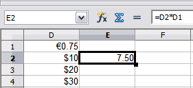
- Input the exchange rate Eur:USD (0.75) in cell D1. Enter amounts (in USD) into cells D2, D3 and D4, for example 10, 20, and 30.
- In cell E2 type the formula =D2*D1. The result is 7.5, correctly shown.
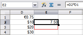
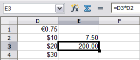
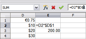
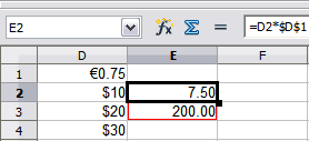
- Copy the formula in cell E2 to cell E3. The result is 200, clearly wrong! Calc has copied the formula using relative addressing - the formula in E3 is =D3*D2 and not what we want which is =D3*D1.
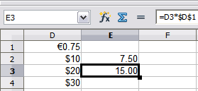
- In cell E2 edit the formula to be =D2*$D$1. Copy it to cells E3 and E4. The results are now 15 and 22.5 which are correct.
Step 2: Setting the exchange rate of Eur at 7.5, then copying it to E3.
Copying formula from E2 to E3 and changing the formula to read absolute reference.
Applying the correct formula from E2 to E3.
The $ signs before the D and the 1 convert the reference to cell D1 from relative to absolute or fixed. If the formula is copied to another cell the second part will always show $D$1. The interpretation of this formula is “take the value in the cell one column to the left in the same row and multiply it by the value in cell D1”.
Cell references can be shown in four ways:
| Reference | Explanation |
|---|---|
| D1 | Relative, from cell E3: the cell one column to the left and two rows above |
| $D$1 | Absolute, from cell E3:the cell D1 |
| $D1 | Partially absolute, from cell E3: the cell in column D and two rows above |
| D$1 | Partially absolute, from cell E3: the cell one column to the left and row 1 |
Knowledge of the use of relative and absolute references is essential if you want to copy and paste formulas and to link spreadsheets.
Order of calculation
Order of calculation refers to the sequence that numerical operations are performed. Division and multiplication are performed before addition or subtraction. There is a common tendency to expect calculations to be made from left to right as the equation would be read in English. Calc evaluates the entire formula, then based upon programming precedence breaks the formula down executing multiplication and division operations before other operations. Therefore, when creating formulas you should test your formula to make sure that the correct result is being obtained. Following is an example of order of calculation in operation.
Table 4 – Order of Calculation
| Left To Right Calculation | Ordered Calculation |
| 1+3*2+3 = 11 | =1+3*2+3 result 10 |
| 1+3=4, then 4 X 2 = 8, then 8 + 3 = 11 | 3*2=6, then 1 + 6 + 3 = 10 |
| Another possible intention could be: | The program resolves the multiplication of 3 X 2 before dealing with the numbers being added. |
| 1+3*2+3 = 20 |
If you intend for the result to be either of the two possible solutions on the left, the way to achieve these results would be to order the formula as:
| ((1+3) * 2)+3 = 11 | (1+3) * (2+3) = 20 |
| Use parentheses to group operations in the order you intend; for example = B4+G12*C4/M12 becoming =((B4+G12)*C4)/M12. |
Calculations linking sheets
Another powerful feature of Calc is the ability to link data through several worksheets. The naming of worksheets can be helpful to identify where specific data may be found. A name such a Payroll or Boise Sales is much more meaningful than Sheet1. The function named SHEET() returns the sheet number in the collection of spreadsheets. There are several worksheets in each book and they are numbered from the left: Sheet1, Sheet2, and so forth. If you drag the worksheets around to different locations among the tabs, the function returns the number referring to the current position of this worksheet.
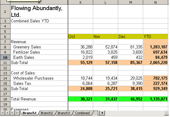
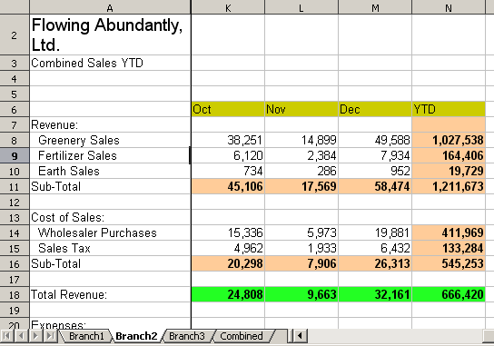
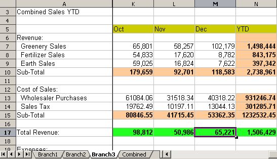
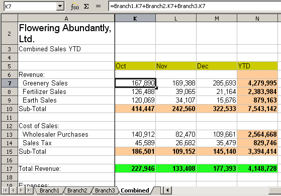
An example of calculations obtaining data from other work can be seen in a business setting where a business combines its branch operations into a single worksheet.
|
Sheet containing data for Branch 1. |
|
Sheet containing data for Branch 2. |
|
Sheet containing data for Branch 3. |
|
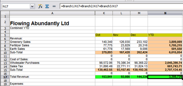
Sheet containing combined data for all branches. |
Combining data from several sheets into a single sheet.
The spreadsheets have been set up with identical structures. The easiest way to do this is to set up the first Branch spreadsheet, input data, format cells, and prepare the formulas for the various sums of rows and columns.
- On the worksheet tab, right-click and select Rename Sheet.... Type Branch1. Right-click on the tab again and select Move/Copy Sheet...
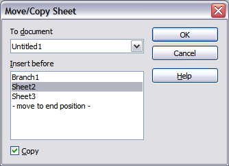
- In the Move/Copy Sheet dialog, select the Copy option and select Sheet 2 in the area Insert before. Click OK, right-click on the tab of the sheet Branch1_2 and rename it to Branch2. Repeat to produce the Branch3 and Combined worksheets.
- Enter the data for Branch 2 and Branch 3 into the respective sheets. Each sheet stands alone and reports the results for the individual branches.
- In the Combined worksheet, click on cell K7. Type =, click on the tab Branch1, click on cell K7, press +, repeat for sheets Branch2 and Branch3 and press Enter. You now have a formula in cell K1 which adds the revenue from Greenery Sales for the 3 Branches.
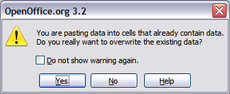
- Copy the formula, highlight the range K7..N17, click Edit > Paste Special, uncheck the Paste all and Formats boxes in the Selection area of the dialog box and click OK. You will see the following message:
- Click Yes. You have now copied the formulas into each cell while maintaining the format you set up in the original worksheet. Of course, in this example you would have to tidy the worksheet up by removing the zeros in the non-formatted rows.
| The Calc default is to paste all the attributes of the original cell(s) - formats, notes, objects, text strings and numbers. |
The Function Wizard can also be used to accomplish the linking. Use of this Wizard is described in detail in the section on Functions.


