Viewing Calc
Using zoom
Use the zoom function to change the view to show more or fewer cells in the window.
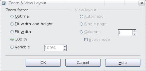
In addition to using the Zoom slider (new in OOo 3.1) on the Status bar, you can open the Zoom dialog and make a selection on the left-hand side.
- Go to the View menu and select Zoom, or
- Double-click on the percentage figure in the status bar at the bottom of the window.
Optimal
Resizes the display to fit the width of the selected cells. To use this option, you must first highlight a range of cells.
Fit Width and Height
Displays the entire page on your screen.
Fit Width
Displays the complete width of the document page. The top and bottom edges of the page may not be visible.
100%
Displays the document at its actual size.
Variable
Enter a zoom percentage of your choice.
Freezing rows and columns
Freezing locks a number of rows at the top of a spreadsheet or a number of columns on the left of a spreadsheet or both. Then when scrolling around within the sheet, any frozen columns and rows remain in view.
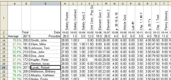
The figure below shows some frozen rows and columns. The heavier horizontal line between rows 3 and 14 and the heavier vertical line between columns C and H denote the frozen areas. Rows 4 through 13 and columns D through G have been scrolled off the page. Because the first three rows and columns are frozen into place, they remained.
You can set the freeze point at one row, one column, or both a row and a column as in the example.
Freezing single rows or columns
- Click on the header for the row below where you want the freeze or for the column to the right of where you want the freeze.
- Select Window > Freeze.
A dark line appears, indicating where the freeze is put.
Freezing a row and a column
- Click into the cell that is immediately below the row you want frozen and immediately to the right of the column you want frozen.
- Select Window > Freeze.
Two lines appear, a horizontal line above this cell and a vertical line to the left of this cell. Now as you scroll around the screen, everything above and to the left of these lines will remain in view.
Unfreezing
To unfreeze rows or columns, select Window > Freeze. The check mark by Freeze will vanish.
Splitting the screen
Another way to change the view is by splitting the window—also known as splitting the screen. The screen can be split horizontally, vertically, or both. You can therefore have up to four portions of the spreadsheet in view at any one time.
Why would you want to do this? Imagine you have a large spreadsheet and one of the cells has a number in it which is used by three formulas in other cells. Using the split screen technique, you can position the cell containing the number in one section and each of the cells with formulas in the other sections. Then you can change the number in the cell and watch how it affects each of the formulas.
Splitting the screen horizontally
To split the screen horizontally:
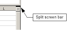
- Move the mouse pointer into the vertical scroll bar, on the right-hand side of the screen, and place it over the small button at the top with the black triangle.
- Immediately above this button you will see a thick black line. Move the mouse pointer over this line and it turns into a line with two arrows.
- Hold down the left mouse button and a grey line appears, running across the page. Drag the mouse downwards and this line follows.
- Release the mouse button and the screen splits into two views, each with its own vertical scroll bar.

Split screen bar on vertical scroll bar with cursor
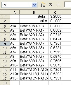
Notice in the split screen example, the ‘Beta’ and the ‘A0’ values are in the upper part of the window and other calculations are in the lower part. You may scroll the upper and lower parts independently. Thus you can make changes to the Beta and A0 values and watch their affects on the calculations in the lower half of the window.
| You can also split the screen using a menu command. Click in a cell immediately below and to the right of where you wish the screen to be split, and choose Window > Split. |
Splitting the screen vertically
To split the screen vertically:
- Move the mouse pointer into the horizontal scroll bar at the bottom of the screen and place it over the small button on the right with the black triangle.
- Immediately to the right of this button is a thick black line. Move the mouse pointer over this line and it turns into a line with two arrows.
- Hold down the left mouse button and a grey line appears, running up the page. Drag the mouse to the left and this line follows.
- Release the mouse button and the screen is split into two views, each with its own horizontal scroll bar.
Removing split views
To remove a split view:
- Double-click on each split line, or
- Click on and drag the split lines back to their places at the ends of the scroll bars, or
- Select Window > Split. This will remove all split lines at the same time.
| Content on this page is licensed under the Creative Common Attribution 3.0 license (CC-BY). |


