FR/Documentation/Calc/Sommes et calculs conditionnels

Cette page est en cours de traduction d'après la page http://wiki.services.openoffice.org/wiki/Documentation/How_Tos/Conditional_Counting_and_Summation dont le lien est dans l'OLH.

Sommes et calculs conditionnels dans in Calc

Ceci est un résumé sur les différentes facon de compter des cellules et de faire a somme de leurs contenu en fonction du résultat de certains tests.

NB

La fonction NB compte le nombre de cellules qui contient des nombres et ignorera les autres. Par exemple les cellules contenant du texte seront ignorées.

NBVAL

La fonction NBVAL compte le nombre de cellules quelque soit leurs contenus (du texte, des nombres, des erreurs, des valeurs logiques ou des formules ). Elle ignore les cellules vides.

NB.VIDE

La fonction NB.VIDE compte le nombre de cellules vides.

SOMME

la fonction SOMME sums all the numbers in the specified cells. See later for how to use it as a conditional function.

SOUS.TOTAL

LA fonction SOUS.TOTAL returns COUNT, COUNTA or SUM results for filtered data, that is data in cells chosen by a filter.

NB.SI

La fonction NB.SI counts those items that meet a single condition. For example COUNTIF(A1:A4; “>4”) counts the cells in A1:A4 that are greater than 4.

SOMME.SI

LA function SOMME.SI sums those items that meet a single condition. For example SUMIF(A1:A4; ”=red”; B1:B4) sums the values in B1:B4 that correspond to “red” entries in A1:A4.

BDNB, BDNBVAL, BDPRODUIT

Les fonction BDNB , fonction BDNBVAL , et fonction BDPRODUIT perform similarly to COUNT, COUNTA and SUM, except that the cells to be counted or summed are chosen according to a table of conditions. For example, DCOUNT(A1:C5; 0; E6:F7) counts the number of rows of A1:C5 for which the multiple conditions specified in E6:F7 are all true.

Conditions dans la selectionn des cellues

One simple method to count or sum using multiple conditions is to enter those conditions in a new row or column. For example, if A1:A6 contains a list of colours and B1:B6 a list of sizes, then we can enter in cell D1 the formula =(A1=”red”), which returns TRUE or FALSE depending if cell A1 is red or not. Alternatively, we can enter in cell D1 the formula =AND(A1=”red”; B1=”big”), which returns TRUE if cell A1 is red AND cell B1 is big and FALSE otherwise. Copy and paste this formula to D2:D6 and we have a range of cells which are TRUE if the conditions are met and FALSE otherwise.

In numerical calculations, TRUE is treated as 1, and FALSE is treated as 0. So entering =SUM(D1:D6) will simply sum those 1s and 0s, and give us the count of items that are both red AND big.

In fact, because TRUE and FALSE evaluate as 1 and 0, we do not need the AND function - in D1 we can simply write =(A1=”red”)*(B1=”big”), and copy/paste down to D2:D6.

Now let us say that C1:C6 contains a list of weights of these items, and we wish to know the total weight for all big red items. In D1 we write =(A1=”red”)*(B1=”big”)*C1, and copy/paste down to D2:D6. D1 will contain the weight in C1 if the conditions are met (and zero otherwise) and so on for D2:D6, Therefore =SUM(D1:D6) will now give us the total weight.

Alternatively, it is possible to fill D1:D6 with an array formula. In D1, write =(A1:A6=”red”)*(B1:B6=”big”)*C1:C6, and enter by pressing Ctrl_Shift_Enter. All the cells in D1:D6 now show the desired weights as before.

SOMMEPROD

The fonction SOMMEPROD can be used to perform the counting and summation calculations in the previous section, without using extra columns. It is necessary to understand array formulas to understand this.

Using the summation example from the previous section, A1:A6=”red”, B1:B6=”big” and C1:C6 may be treated as 3 separate arrays, not displayed but internally calculated.

=SUMPRODUCT(A1:A6=”red”; B1:B6=”big”; C1:C6) will multiply corresponding elements of the arrays together and return their sum, i.e.:

(A1=”red”)*(B1=”big”)*C1 + (A2=”red”)*(B2=”big”)*C2 + ...

This again gives us the total weight, without requiring an extra column.

Notice that SUMPRODUCT formulas are simply entered by pressing the Enter key - they do not require Ctrl_Shift_Enter even though arrays are involved.

Also, be aware that calculations using very large arrays take a lot of computer processing time, and may slow the spreadsheet down.

SOMME with array formulas

An alternative to SUMPRODUCT is to use the SUM function. The previous example would be written:

=SUM( (A1:A6=”red”)*(B1:B6=”big”)*C1:C6) )

and entered as an array formula by pressing Ctrl_Shift_Enter. As with SUMPRODUCT, this works by multiplying corresponding elements of the arrays together and returning their sum.

DataPilot

Another way to approach conditional counting and summation is to use the DataPilot to generate an interactive table, whereby data can be arranged and summarised according to different points of view.

Trucs et Astuces: checking settings

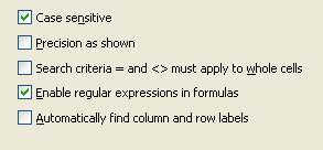
When matching text with some functions (such as SUMIF) , the results may well depend on the settings on the Tools menu-> Options-> OpenOffice.org Calc-> Calculate page. If the user's settings are incorrect, the results may therefore be wrong.

One solution is to include prominently in the spreadsheet a check that the settings are correct. For example:

=IF(ISERR(SEARCH(".";"a"));"ERROR: please enable regular expressions";"")

will show an error message if regular expressions are disabled.

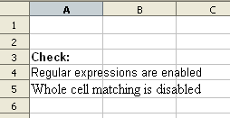
Another example - in cell A3 enter the text:

Check: 

In cell A4 enter:

="Regular expressions are "&IF(COUNTIF(A3;".*"); "enabled"; "disabled")

In cell A5 enter:

="Whole cell matching is "&IF(COUNTIF(A3;"<>e"); "enabled"; "disabled")

or better, use appropriate error messages.

Trucs et Astuces: items between two dates

Dates are stored internally as numbers and can thus be compared easily. For example, to count the number of cells in A1:A6 between two dates, you could use:

=SUMPRODUCT(A1:A6>DATEVALUE("5 Nov 06"); A1:A6<DATEVALUE("5 Dec 06"))

If you express the dates with slashes (e.g. “1/2/2005”) you can dispense with the DATEVALUE function, as Calc will convert the date. However, be aware that in one country this text may be converted to 1Feb05 and in another to 2Jan05.

Trucs et Astuces: summing the largest/smallest items

To add up the largest 3 numbers in A1:A5, the most straightforward method is to enter:

=LARGE(A1:A5; 1) in cell B1

=LARGE(A1:A5; 2) in cell B2

=LARGE(A1:A5; 3) in cell B3

so that the largest 3 numbers are in B1:B3, and then use the formula:

=SUM(B1:B3) to give the result.

This method is very clear, and generally therefore to be recommended.

However if you wish to derive the same result in a single cell, you could use

=SUMPRODUCT(LARGE(A1:A5; ROW(A1:A3)))

Here ROW(A1:A3) is a 1 column 3 row array containing the numbers 1, 2, 3.

LARGE(A1:A5; ROW(A1:A3)) is then a 1 column 3 row array containing the largest 3 numbers and SUMPRODUCT simply adds them up. We could use SUM instead of SUMPRODUCT but in that case the formula must be entered as an array formula by pressing Ctrl_Shift_Enter.

To add up the largest 4 numbers (say), use ...ROW(A1:A4).. instead of ...ROW(A1:A3)..

To add the smallest numbers, use SMALL(...) instead of LARGE(...).

Trucs et Astuces: summing matching blank, etc cells

=SUMPRODUCT(ISBLANK(A1:A5); B1:B5)

sums those cells in B1:B5 corresponding to blank cells in A1:A5.

Other similar functions (e.g. ISTEXT, ISNUMBER) can be used in the same way.

Trucs et Astuces: summing more than one column

=SUMPRODUCT(D1:D6="red";E1:E6+F1:F6)

will sum cells in E1:E6 and in F1:F6 which correspond to cells in D1:D6 containing red. For example if D2 and D4 contain red, the result is E2+F2+E4+F4.

Trucs et Astuces: summing every nth row

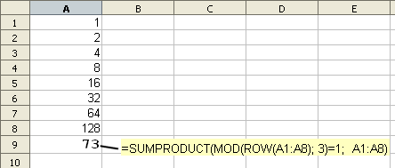
=SUMPRODUCT(MOD(ROW(A1:A8); 2)=0;  A1:A8)

will sum every second row in A1:A8. Change the =0 to =1 to sum every second row, but starting at the first row. Change the 2 to 3 to sum every third row, and so on.

Trucs et Astuces: summing items with certain formatting

The CELL function returns information about cells, for instance the format that numbers or dates are displayed in and the column width. It can thus be used with one of the methods above. There is no function that returns the colour or font of a cell. If no independent formula relating to colour or font exists, then it may be necessary to use a macro.

Trucs et Astuces: summing matching items in a separate list

Say that A1:A9 contains a list of dates, B1:B9 contains phone numbers and C1:C9 the costs of making phone calls. F1:F5 is a list of certain phone numbers, and you want to know the total cost of calls to these numbers.

In cell D1 enter:

=ISNUMBER(MATCH(B1; F$1:F$5; 0))*C1

and copy/paste down to D2:D9

=SUM(D1:D9) now gives the total cost of calls.

To perform this calculation without an extra column, you could use:

=SUMPRODUCT(NOT(ISERROR(MATCH(B1:B9; F$1:F$5; 0))); C1:C9)

We discussed above how it can be important to check Calc settings; this is a good example - if the user has regular expressions turned on (the default) a telephone number written as (720) 528-1700 is interpreted as a regular expression and might match entries other than (720) 528-1700.

Content on this page is licensed under the Public Documentation License (PDL).