Using other "what if" tools

OpenOffice.org 3 Calc Guide

Chapter 9 Data Analysis

< Previous Section

Next Section >

• Consolidating data
• Creating subtotals
• Using scenarios
• Multiple operations
• Goal seek
• Solver

< Previous Page

Next Page >

Like scenarios, Data > Multiple Operations is a planning tool for “what if” questions. Unlike a scenario, the Multiple Operations tool does not present the alternate versions in the same cells or with a drop-down list. Instead, the Multiple Operations tool creates a formula array: a separate set of cells showing the results of applying the formula to a list of alternative values for the variables used by the formula. Although this tool is not listed among the functions, it is really a function that acts on other functions, allowing you to calculate different results without having to enter and run them separately.

To use the Multiple Operations tool, you need two arrays of cells. The first array contains the original or default values and the formulas applied to them. The formulas must be in a range.

The second array is the formula array. It is created by entering a list of alternative values for one or two of the original values.

Once the alternative values are created, you use the Multiple Operations tool to specify which formulas you are using, as well as the original values used by the formulas. The second array is then filled with the results of using each alternative value in place of the original values.

The Multiple Operations tool can use any number of formulas, but only one or two variables. With one variable, the formula array of alternative values for the variables will be in a single column or row. With two variables, you should outline a table of cells such that the alternative values for one variable are arranged as column headings, and the alternative values for the other variable act as row headingss.

Setting up multiple operations can be confusing at first. For example, when using two variables, you need to select them carefully, so that they form a meaningful table. Not every pair of variables is useful to add to the same formula array. Yet, even when working with a single variable, a new or tired user can easily make mistakes or forget the relation between cells in the original array and cells in the formula array. In these situations, Tools > Detective can help to clarify the relations.

You can also make formula arrays easier to work with if you apply some simple design logic Place the original and the formula array close together on the same sheet, and use labels for the rows and columns in both. These small exercises in organizational design will make working with the formula array much less painful, particularly when you are correcting mistakes or adjusting results.

If you export a spreadsheet containing multiple operations to Microsoft Excel, the location of the cells containing the formula must be fully defined relative to the data range.

Multiple operations in columns or rows

In your spreadsheet, enter a formula to calculate a result from values that are stored in other cells. Then, set up a cell range containing a list of alternatives for one of the values used in the formula. The Multiple Operations command produces a list of results adjacent to your alternative values by running formula against each of these alternatives.

Before you choose the Data > Multiple Operations option, be sure to select not only your list of alternative values but also the adjacent cells into which the results should be placed.

In the Formulas field of the Multiple operations dialog, enter the cell reference to the formula that you wish to use.

The arrangement of your alternative values dictates how you should complete the rest of the dialog. If you have listed them in a single column, you should complete the field for Column input cell. If they are along a single row, complete the Row input cell field. You may also use both in more advanced cases. Both single and double-variable versions are explained below.

The above can be explained best by examples. Cell references correspond to those in the following figures.

Let’s say you produce toys that you sell for $10 each (cell B1). Each toy costs $2 to make (cell B2), in addition to which you have fixed costs of $10,000 per year (cell B3). How much profit will you make in a year if you sell a particular number of toys?

Calculating with one formula and one variable

1. To calculate the profit, first enter any number as the quantity (items sold); in this example, 2000 (cell B4). The profit is found from the formula Profit=Quantity * (Selling price – Direct costs) – Fixed costs. Enter this formula in B5: =B4*(B1-B2)-B3.
2. In column D enter a variety of alternative annual sales figures, one below the other; for example, 500 to 5000, in steps of 500.
3. Select the range D2:E11, and thus the values in column D and the empty cells (which will receive the results of the calculations) alongside in column E.
4. Choose Data > Multiple Operations.
5. With the cursor in the Formulas field of the Multiple operations dialog, click cell B5.
6. Set the cursor in the Column input cell field and click cell B4. This means that B4, the quantity, is the variable in the formula, which is to be replaced by the column of alternative values. The figure below shows the worksheet and the Multiple operations dialog.


Sheet and Multiple operations dialog showing input
7. Click OK. The profits for the different quantities are now shown in column E.


Sheet showing results of multiple operations calculations

You may find it easier to mark the required reference in the sheet if you click the Shrink icon to reduce the Multiple operations dialog to the size of the input field. The icon then changes to the Maximize icon; click it to restore the dialog to its original size.

Calculating with several formulas simultaneously

1. In the sheet from the previous example, delete the contents of column E.
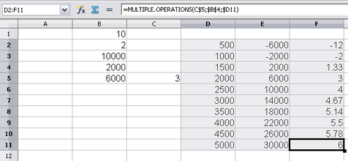
2. Enter the following formula in C5: =B5/B4. You are now calculating the annual profit per item sold.
3. Select the range D2:F11, thus three columns.
4. Choose Data > Multiple Operations.
5. With the cursor in the Formulas field of the Multiple operations dialog, select cells B5 and C5.
6. Set the cursor in the Column input cell field and click cell B4. The figure below shows the worksheet and the Multiple operations dialog.


Sheet and dialog showing input
7. Click OK. Now the profits are listed in column E and the annual profit per item in column F.


Results of multiple operations calculations

Multiple operations across rows and columns

You can carry out multiple operations simultaneously for both columns and rows in so-called cross-tables. The formula must use at least two variables, the alternative values for which should be arranged so that one set is along a sinle row and the other set appears in a single column. These two sets of alternative values will form column and row headings for the results table produced by the Multiple Operations procedure.

Select the range defined by both data ranges (thus including all of the blank cells that are to contain the results) and choose Data > Multiple operations. Enter the cell reference to the formula in the Formulas field. The Row input cell and the Column input cell fields are used to enter the reference to the corresponding cells of the formula.

Beware of entering the cell reference of a variable into the wrong field. The Row input cell field should contain not the cell reference of the variable which changes down the rows of your results table, but that of the variable whose alternative values have been entered along a single row.

Calculating with two variables

You now want to vary not just the quantity produced annually, but also the selling price, and you are interested in the profit in each case.

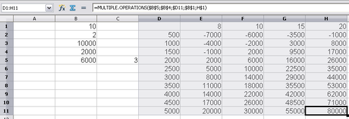
Expand the table shown above. D2 thru D11 contain the numbers 500, 1000 and so on, up to 5000. In E1 through H1 enter the numbers 8, 10, 15 and 20.

1. Select the range D1:H11.
2. Choose Data > Multiple Operations.
3. With the cursor in the Formulas field of the Multiple operations dialog, click cell B5 (profit).
4. Set the cursor in the Row input cell field and click cell B1. This means that B1, the selling price, is the horizontally entered variable (with the values 8, 10, 15 and 20).
5. Set the cursor in the Column input cell field and click cell B4. This means that B4, the quantity, is the vertically entered variable.


Sheet and dialog showing input
6. Click OK. The profits for the different selling prices are now shown in the range E2:H11.


Results of multiple operations calculations