Differences in Use between Calc and Excel
- Introduction
- Sharing Files with Microsoft Office Users
- Importing other Microsoft Office Files
- General Differences in Use between OpenOffice.org and Microsoft Office
- Differences in Use between Writer and Word
- Differences in Use between Calc and Excel
- Differences in Use between Impress and PowerPoint
- Customizing OpenOffice.org
This chapter summarizes the differences in use between OpenOffice.org Calc 2.0 and Microsoft Excel (various versions). The information in this chapter builds upon the information given in Chapter General Differences in Use between OpenOffice.org and Microsoft Office.
The Calc interface
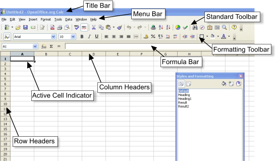
The main Calc workspace is shown below.
Terminology
Table below summarizes some terminology differences between Calc and Excel.
All of the chapters in this guide and in the Calc Guide use the AOo Calc terminology.
| Object | Excel | Calc |
|---|---|---|
| Individual cell (A1) | Cell | Cell |
| Entire file | Workbook | Spreadsheet |
| One tabbed sheet in a workbook (Sheet 1) | Worksheet | Sheet |
| Callouts in cells which appear when the mouse pointer is positioned over the cell | Comments | Notes |
User interface
Calc uses a Single Document Interface (SDI). This means that each document has its own window in which only one document is displayed at a time. Excel uses a Multiple Document Interface (MDI) where all open documents are displayed within one parent window. When you close the parent window, all files are also closed.
Two of Calc’s strong points are the accessibility of information about the active document and the ease of navigation of an SDI. Each Calc window provides menus, toolbars and other features that directly relate to the document open in that window.
When more than one OpenOffice.org document is open, you can switch between the active document and other open documents in several ways:
- From the Window menu, select the document you want to become active.
- Use the Restore Down button on the Title Bar to minimize the active document and reveal other open documents.
- Select a document from your desktop’s Panel or Taskbar to activate it.
- Close the current document to access other open documents.
- Use the Alt+Tab shortcut keys to cycle through the open documents.
Drag and drop
Drag and drop works slightly differently in Calc than it does in Excel:
- In Excel, after you select the cell or range to be moved, you need to position the pointer fairly precisely on the border of the cell or range for drag and drop to be available. In Calc, after selecting the cell or range, you can position the pointer anywhere within the range.
- In Calc, to drag and drop a single cell, do this:
- Select the cell.
- Drag to select at least one additional cell.
- Drag back so that only the desired cell is selected. Then the cell can be dragged and dropped.
- In Calc, to leave the source cell or range intact while dragging and dropping (in other words, to create a copy of the source cell or range), first drag in the normal way, then just before dropping, press and hold the Ctrl key, then release the mouse button.
Keyboard shortcuts
| Function | Excel Shortcut | Calc Shortcut |
|---|---|---|
| Rearranges the relative or absolute references (for example, A1, $A$1, $A1, A$1) in the input field | F4 | Shift+F4 |
| Edit cell comment (known as “notes” in Calc) | Shift+F2 | Control+F1 |
| Fill right or Fill down | Control+R or Control+D | No equivalent |
| Go to specific cell | F5 | F5 (shows Navigator) |
| Insert Function | No standard equivalent | Control+F2 |
| Enter into all currently selected cells | Control+Enter | Alt+Enter
Alt+Shift+Enter (also applies the cell format) In both cases cells must be contiguous. |
Range lists
Excel allows all parameters to be range lists. Some examples are:
=SUM(A1,A3) is the sum of two cells (function has 2 parameters).
=SUM((A1,A3)) is the same, but with one parameter being a range list.
=INDEX((A2:A3,C2:C3),1,1,2)
Calc only allows range lists in the INDEX function. For example:
=INDEX((A2:A3;C2:C3);1;1;2) returns the first cell of the second range in the range list.
Deleting cell contents
In Excel, pressing the Delete key instantly deletes the contents of the cell. In Calc, pressing Delete calls up a dialog box where you can specify what to delete:
- Strings
- Numbers
- Date & Time
- Formulas
- Comments
- Formats
- Objects
The items checked by default are: Strings; Numbers; Date & Time; Formulas; and Comments. Thus, pressing Delete and then Enter will delete the items checked by default.
You can bypass the dialog and instantly delete the items checked by default by pressing the Backspace key rather than the Delete key.
Filling down or to the right
Using the Fill Down (or Fill Right) feature
In Excel, it is possible to copy and paste a cell to a range of cells below or to the right of the target cell by selecting a range, with the source cell at the top (when filling down) or at the left (when filling to the right); then use the keyboard shortcut Ctrl+D (to fill down) or Ctrl+R (to fill to the right). There is also a menu path that accomplishes the same task as the keyboard shortcuts.
In Calc, the same features are available, but only through a menu path, not through keyboard shortcuts. Also, in Calc, it is possible to fill up and to the left. The menu path is: Edit > Fill > Down (or Up, Right, or Left).
Using the fill handle
In both Calc and Excel, the fill handle can be used to copy contents of a cell down or to the right. This feature works somewhat differently between Calc and Excel.
To use the fill handle, select the source cell, position the pointer over the fill handle so it becomes a small plus sign, and then drag either down or to the right.
- In Excel, the above action will copy the contents of the cell.
- In Calc, if the source cell contains only letters, or a string of letters and numbers but not ending in a number (example: A4B), then the source cell will be copied exactly.
- If the cell is numeric, the number will increment by 1 with each additional cell (example: 5, 6, 7, ...; or 1.5, 2.5, 3.5, ...). If the source entry is a string which begins with or ends with a number, the number component of the string will increment by 1 (example: A1, A2, A3, ...).
- In Calc, it is possible to copy the source cell exactly, without incrementing, by holding the Ctrl key while clicking the fill handle and dragging.
In either Excel or Calc, if there are two adjacent cells which contain numerical entries, selecting both cells and then using the fill handle to extend the series will result in the same increment between the “filled” cells as was present between the two source cells. For example, if cell A1=1.0 and cell A2=1.1, selecting these cells and using the fill handle will yield: A3=1.2; A4=1.3; etc.
Default number format
Calc and Excel use different default number formats.
- With Excel, the cells are set to the “General” category number format., so if you entered 25.12345 in a cell it would display “25.12345”.
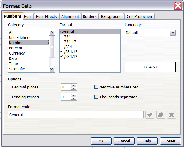
- In Calc a default formatted cell is set to the “Number” category in the “General” format. Thus, if 25.12345 is entered, 25.12 will be displayed.
Interpreting cell contents
In Calc if a cell is defined as text, even if the cell contains a number, then that cell is treated as text, which means it has the numeric value zero for formulas.
For example, if cell A1 is formatted as text and contains the character “1”, in Excel a formula =A1+1 would return the value 2, but in Calc it would return the value 1.
In functions, such an entry will be ignored rather than treated as zero. For example, the function AVERAGE will not treat a text entry as zero, but will ignore it. If cell A1 is a text entry of “1”, and cell A2 is a numerical entry of “10”, =AVERAGE(A1:A2) would be 10, not 5.
Limitations
The maximum number of sheets in Calc is 256. In Excel, the number of sheets according to the Microsoft website is “Limited by available memory (default is 3 sheets)”.
Form fields
List boxes in Calc can either have multi-selection or not, whereas Excel has two multi-selection modes: multi and extend. In Excel a multi-selection listbox’s link to a cell is ignored. In Calc the link works, but if more than one item is selected the cell’s value is set to #N/A.
In Calc each option button has its own link to a cell, setting its value to true or false depending on whether the option is selected. In Excel the cell link returns the number of the selected option button.
Relative addressing of sheets
In Calc it is possible to have relative addressing of sheets. As with column and cell references, the dollar sign is used to signify that the sheet name is absolute.
=$Sheet2!$A$1 always refers to the first cell on sheet 2.
=Sheet2!$A$1 when on sheet one and copied to another sheet will refer to the first cell of the next sheet.
This is not possible in Excel.
Named ranges and “Natural Language” formulas
It is possible, in some versions of Excel, to have the same range name on different sheets. This is not possible in Calc. However, if the duplicated range name in Excel refers to the same cell in each case, then it can be simulated in Calc with a range name without the sheet being specified and thus the range name refers to the specified cell on the current sheet.
Calc does have Natural Language. This is where column or row labels are used (without defining them as range names) in a formula. In Excel, to refer to a cell, a space is used between the label names. In Calc an exclamation mark “!” (sometimes called pling) is used.
In Calc the names are enclosed in single quotes (done automatically by Calc if the label starts with a letter and only has alphanumeric characters). To turn this feature on or off use: Tools > Options > Spreadsheet > Calculate > Automatically find column and row labels.
Array formulas
Calc supports array formulas (formulas entered using Ctrl + ⇧ Shift + ↵ Enter ), but Calc can not have array constants in a formula. The work-around is to have the constant values in cells on a sheet and refer to them.
Some Excel array formulas seem to rely on the way that Excel is calculating a result in a non-documented way–such a practice is not a good idea even within Excel only, and certainly not a good idea when importing a file containing such a formula into Calc.
Functions
Optional parameters in functions
Some formulas have more than one optional parameter at the end of the parameter list. In Excel it is possible to leave an optional parameter blank and specify a later parameter, but this is not possible in Calc. When using Calc functions, parameters marked as "optional" can be left out (or left empty) only when no parameter follows.
For example, to calculate an annuity by using the Present value function, PV(Rate; NPER; PMT; FV; Type), without the Future Value variable (FV):
- In Excel the formula =PV(0.05,10,100,,1) returns -$810.78
- in Calc =PV(0.05;10;100;;1) returns Err:511 (Variable missing).
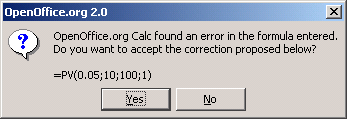
When you enter the PV function in Calc with the FV variable empty, a message box is displayed offering to change the incorrect input to "=PV(0.05;10;100;1)":
This, too, is incorrect as it will produce a value of -772.79.
The work-around is to put values in for the missing parameters. For the above example, putting a zero in for the blank parameter returns the correct result for the annuity, -$810.78.
Date values in financial functions
In Excel some of the financial functions accept string parameters for dates; in Calc financial functions require a serial number, although you can simply type in the dates in date format without quotes.
Analysis Addin functions
Whenever an Excel Analysis ToolPak function has the same name as a Calc function, there is an equivalent in the Calc Analysis AddIn function but with a trailing _ADD. This ensures compatibility with Excel but without changing the behavior of Calcs built-in functions.
For example, the functions EFFECT and CONVERT provided by the Excel Analysis ToolPak are named EFFECT_ADD and CONVERT_ADD in Calc and return the same results.
The functions whose names end with _ADD return the same results as the corresponding Microsoft Excel functions. Use the functions without _ADD to get results based on international standards. For example, the WEEKNUM function calculates the week number of a given date based on international standard ISO 6801, while WEEKNUM_ADD returns the same week number as Microsoft Excel.
Differences in function results
Calc and Excel handle the missing Reference parameter with the Cell function, CELL(Info_type; Reference), differently. If Reference is missing, Calc uses the position of the cell in which this formula is located. Excel uses the reference of the cell in which the cursor is positioned.
Functions not implemented or imported
Excel functions which are not imported or implemented in Calc include INFO and GETPIVOTDATA. Excel has no equivalent for Calc’s ARABIC function which calculates the value of a Roman number.
There are issues when importing both the Ceiling function, CEILING (Number; Significance; Mode), and the Floor function, FLOOR(Number; Significance; Mode). If both parameters Number and Significance are negative and the Mode value is equal to zero or is not given, the results in OpenOffice.org and Excel will differ after the import has been completed. If you are exporting a Calc spreadsheet to Excel, use Mode=1 to see the same results in Excel as in Calc.
Pivot Table
Pivot Tables exist in Calc as well as in Excel. They were renamed in earlier Calc from DataPilot to Pivot Table. However, there are a number of limitations. Pivot tables import from Excel into Calc (although the cells do not have the PivotTable shading), but as soon as they are worked on these limitations become apparent.
The limitations are:
- There is no PivotChart facility, but a DataPilot can be used as the data source for a chart.
- The user interface allows a maximum of 8 fields in the data, row or column areas. (An alternative interface which allows more is available from http://homepages.paradise.net.nz/hillview/OOo/ in a document called MyDataPilot.sxc).
- There is some ability to group data (for example, a date field grouping by week or quarter but not by month). The work-around is to create a new column with a formula for calculating the grouping, for example =Month().
- You can not define different formats for different fields.
- Calc can have formulas based on things like “Difference From” or “% of”, but can not have its own custom fields (work-around, create new columns to calculate the desired values).
- The Application Program Interface specification is incomplete for writing macros that work with Pivot tables—for example; the ability to control, through another program such as Apache OpenOffice's own macro language BASIC, whether the tables have grand totals or have access to Pivot tables created from external data.
AutoFilter
There are a number of AutoFilter differences between Excel and Calc:
- There is only one AutoFilter active at a time, for a spreadsheet document, unless using database range names. The rows remain hidden but the drop-downs in the first row disappear on applying AutoFilter elsewhere. To have more than one AutoFilter active at the same time, define a database range name (Data > Define Range) for the data, then it is possible to have more than one AutoFilter active on the one sheet (which Excel can not do.)
- The remaining visible row numbers do not change color to warn you that there is a filter in place.
- Error values do not show as an option in the drop-down lists when cells in the column have errors.
- In the drop-down lists, the equivalent to Excel’s “Custom” is called “Standard.”
- The top 10 in the drop-down list is literal, but to get the same degree of control you can use Standard and specify “largest”, “largest%”, “smallest” or “smallest%” in the condition field.
- Use regular expressions to specify criteria to select rows based upon the text in the cells. To do this:
-
- Choose “Standard” from the drop-down list.
- Click More so that the rest of the dialog is displayed.
- Check Regular expressions.
Table 16 has some examples to help an Excel user use regular expressions.
| Excel custom command | Comparison Field | Equivalent Regular Expression |
|---|---|---|
| Begins with x | = | ^x.* |
| Does not begin with x | <> | ^x.* |
| Ends with x | = | .*x$ |
| Does not end with x | <> | .*x$ |
| Contains x | = | .*x.* |
| Does not contain x | <> | .*x.* |
You are not limited to these regular expressions. They are included here to show how to achieve the same result for AutoFilter in Calc as can be achieved in Excel.
Inserting comments
In Excel, a comment could be added by right-clicking on a cell and selecting Insert Comment from the context menu. Also, a comment in Excel can be edited or deleted by right-clicking on the cell.
In Calc, there is no context menu selection for inserting a comment. A comment is inserted by the menu path Insert > Comment.
To edit an existing comment in Calc, the same menu path is used (Insert > Comment).
To delete a comment in Calc, either:
- Select Insert > Comment, then highlight and delete the contents of the note; or
- Press Delete; then from the dialog box, uncheck all items except for Comments.
Solver
OOo versions prior to v3.0 had no equivalent in Calc to the Solver add-in for Excel.
V3.0 and above do have a Solver under: Tools → Solver.
The issue was discussed here Issue 8808 .
Charts
Chart types that Excel provides that Calc does not:
- Bar of pie converts to a 2D - columns - normal
- Pie of pie converts to a 2D - columns - normal
- Radar filled converts to line radar
- Radar with markers–converts to 2D–net–normal but counter clockwise rather than Excel’s clockwise
- Bubble charts convert to XY charts
- Surface Charts convert to Deep 3D bar charts
Other charting issues include:
- Charts are slower to update in Calc than in Excel.
- There are fewer axis options, such as no option for having an inverted y axis (negative at top towards positive at bottom).
- The data must be contiguous, with the labels in the first row or column.
- To change the range, click on the border of the chart so that it is selected (green selection points) > Right Click > Modify Data Range...
Number formats
There is no “accounting” format (with the currency symbol at the left edge of the cell).
There is no predefined option for bracketing negative numbers. Use a custom format such as “$#,##0.00_);[RED]($#,##0.00)”.
Use of Autosum feature
The Autosum feature (invoked by clicking on the upper-case Greek sigma) works slightly differently in one respect in Calc than in Excel.
For either Excel or Calc, you can select an empty cell, generally just below the bottom of a range containing numbers to be summed (or to the right of a range of numbers to be summed). When the Autosum button is clicked, Excel or Calc will propose a range to be summed, which in many cases, is in fact the range the user intended. If this is the correct range, pressing Enter will enter the SUM function into the cell. If the proposed range is not what the user intended, the user can highlight the range desired, then press Enter. There is no difference between Excel and Calc when using the Autosum as described above.
In Excel, you can also first highlight the range to be summed plus one additional blank cell, then click Autosum. The SUM function will then be entered in the previously blank cell. This use of Autosum is not available in Calc.
Grid lines and other view settings
In Excel grid lines on the screen are a property of a Worksheet. In Calc it is a document-wide property, set as follows:
Tools > Options > OpenOffice Calc > View
Hidden rows
There is no “select only visible rows” command. Selecting a block of cells with hidden rows and deleting will delete the hidden rows as well. Work-around: select each visible row manually before deleting. See IannzGotoSpecial.sxc, available from former http://homepages.paradise.net.nz/hillview/OOo/IannzGotoSpecial.sxc, for a macro that can select only the visible cells.
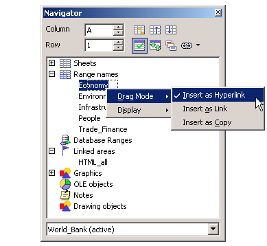
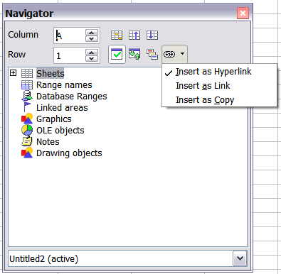
Apache OpenOffice’s Navigator (Figure 3) provides a hierarchical view of the objects that make up a document. With the Navigator you can view a listing of objects such as sheets, range and database names, linked areas, graphics, OLE objects, notes and drawing objects. While it is a convenient way to browse and select the various objects that make up a document, you can also use it to copy cells or insert links into a spreadsheet from another document, or from a sheet within the same spreadsheet. (See Working across spreadsheets.)
The Navigator copies and inserts links using drag and drop. To use the Navigator to create a link, the data to be linked must be defined as a named range within the source document. If there are no named ranges within the source document, the Navigator will not list any linkable items.
The Navigator also displays the objects and can link data from Excel spreadsheets.
Styles and Formatting window
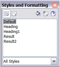
Calc has two types of styles, cell and page. To display the Styles and Formatting window, press F11 or select Format > Styles and Formatting. Right-click in the Styles and Formating window to create, modify, or delete styles.
Conditional formatting and styles
Conditional formating requires styles to be defined before selecting Format > Conditional formatting.
Function list
The Function list is a floating or dockable window that provides information about the available functions. It is an alternative to Functions Wizard. To view it: Insert > Function List.
Error values
Some functions in Calc return cryptic error messages like Err:503. To get a message that is more meaningful, you can select the cell with the error message, then look at the right end of the status bar. In this case, it will show “Error: Invalid floating point operation” (for example, division by zero).
A full description for each error message is given in the OpenOffice Help.
Working across spreadsheets, web pages and database data
Working across spreadsheets
Calc’s Navigator can be used to copy or link to data from another spreadsheet (source).
To insert a link (or reference) to or copy a cell or range of cells with the Navigator:
- Open the source and the target documents.
- Open the Navigator from the target document. Use the Edit > Navigator command or the F5 shortcut. Select the Drag mode you want to use (see ).
- Insert as Hyperlink - creates a hyperlink back to the source file.
- Insert as Link – insert a linked copy of the data in the target document.
- Insert as Copy – copies the range to the target document, but does not link it to the source range.
- Select the source document from the box at the bottom of the dialog.
- Browse to the Range names category and open it by clicking on the plus (+) sign. If there are no named ranges in the source document there will be no ranges available for insertion.
- Select and drag the range you want to link to the target sheet.
To refer to the contents of cells in another spreadsheet document, or workbook, the syntax is 'url of other workbook'#$sheetname.cellrange. For example, on a Linux system:
'file:///home/hillview/Documents/Tests/Address.xls'#$Sheet1.A1
or, on a Windows system:
'file:///C:/Documents/Tests/Address.xls'#$Sheet1.A1
To input these links, you can:
- Type in the formula up to the point where the link is required.
- Select Window > [to select the desired document].
- It is not obvious that this is working, but it is. Select the desired cell or range of cells.
- Select Window > [select the original document].
- Finish entering the formula.
What is disconcerting is that the value displayed is based on the value of the cell (or range of cells) when the linked document was last saved.
So, to check it, save the linked document and update the link in the document (Edit > Links) that contains the link.
To have persistent updating of data between two spreadsheets, insert Dynamic Data Exchange (DDE) links:
- Select and copy the range of cells to be linked to.
- Change to the spreadsheet that requires the link and select the
- Open the Paste Special dialog, Edit > Paste Special and check the Link option (the checkbox at the bottom left of the dialog).
- Click OK to insert the DDE link.
These cells will have a persistent link to the contents of the other sheet and the values returned can then be used in other formulas.
Links to HTML data or other spreadsheets
To link to data on the Internet:
- In a browser navigate to the desired page.
- Copy the URL.
- In Calc, Insert > Link to External Data.
- Paste in the URL.
- This step is not obvious: press Enter, wait a moment and the bottom list box (called Available tables/ranges) will show:
- HTML_all (the entire page)
- HTML_tables (all the tables on the page)
- HTML_1 (each table consecutively numbered on the page)
- Select the desired option from the list box.
- Optionally check the Update every checkbox and specify how often to update.
The same process can be used for linking to data in spreadsheets.
| The source file must be saved before the update can take place. (In AOo, AutoSaves overwrite the original file, so with AutoSaves turned on, this feature could be more useful than it first appears.) |
Links to database data
- Display the Data source viewer (F4).
- In the Data Explorer window, navigate to the desired table or query (if it is not visible click Explorer on or off–left button in the Data source toolbar).
- Drag the table or query onto the sheet. (See Chapter 11, “Getting Started with Base” in the Getting Started guide for information about working with data sources, such as registering the data source.)
Printing
Calc and Excel have similar printing functionality, but there are some important differences.
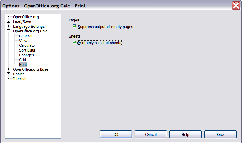
By default, Excel only prints the active sheet. By contrast, Calc will print all of the sheets in the spreadsheet by default. To direct Calc to only print the active sheets, go to Tools > Options > OpenOffice Calc > Print. Check the box Print only selected sheets. You can also check the box Suppress output of empty pages.
| We recommend selecting both boxes, to print only selected sheets and to suppress output of empty pages. |
By default, if no print ranges have been specified anywhere within the spreadsheet, the print range within a sheet will be chosen as a rectangular area from cell A1, to the lowest right cell that has content.
If a print range has been specified within the spreadsheet, even on a different sheet, there is no longer a default print range on any of the sheets. If no print range is established for a particular sheet, nothing from that sheet will be printed.
If you only want a portion of the spreadsheet to print, you must first specify a print range.
To define the print range (this is the equivalent of File > Page Setup > Sheet in Excel, first three fields):
- Format > Print Ranges > Edit.
- In the Edit Print Ranges dialog, select the desired range for each of the fields.
- You can select noncontinuous areas for the print area, with each area being on a separate page. Each area is separated by a semicolon.
Calc provides a page-break view.
- View > Page break preview
Other settings, such as whether to have grid-lines, are done through the page style:
- Format > Page > Sheet
Print preview:
With Excel, a print preview will show what will actually be printed when finally sent to the printer with the present settings in place. With Calc, the print preview will show the print ranges from all the sheets in the spreadsheet, even if it has been specified to only print active pages.
To print:
- File > Print.
- Click Options to change the settings for suppressing blank pages or only the selected sheets.
- Other settings are the same as in Excel.
Macros
Macros written in VBA for Excel do not work in Calc and macros written in StarBasic for Calc do not run on Excel. Re-writing of macros is required when moving spreadsheets between either application.
Some additional resources for writing Basic macros include:
“Porting Excel/VBA to Calc/StarBasic” http://documentation.openoffice.org/HOW_TO/various_topics/VbaStarBasicXref.pdf
StarOffice 8 Programming Guide for BASIC
“Useful Macro Information for OpenOffice”, by Andrew Pitonyak, https://pitonyak.org/AndrewMacro.odt
OpenOffice.org Macros Explained, by Andrew Pitonyak, available from the publisher: https://www.hentzenwerke.com/catalog/oome.htm or from various online booksellers.
Andrew Pitonyak’s web site for AOO macros: https://pitonyak.org/oo.php
Number recognition
Number recognition is where the user types in a “number” and the format of the cell changes accordingly. The same thing applies to text copied from outside Calc and pasted into a spreadsheet.
Rather than compare and contrast Excel with Calc, this section outlines how number recognition works in Calc (which is slightly different from Excel).
Number recognition is dependent on locale. To set the default locale for AOo, use Tools > Options > Language Settings > Languages.
To set the locale for particular cells, select the cells, right-click, and select Format > Cells > Numbers tab > Language.
Default cell formats
The default cell formats are given in Table 15. To determine the default for a locale:
- Select a cell that has not been formatted.
- Select Format > Cells > Numbers tab.
- Click on the desired category.
- Look for the default named in the Format and Format codes portion of the dialog.
| Category | Default format | Format changed when input is different category? |
|---|---|---|
| Number | General | Yes |
| Date | Two defaults based on locale, one for date only and another for date and time. | Yes |
| Time | Default for the locale | Yes |
| Boolean | TRUE or FALSE | Yes |
| Percentage | 0.00% | No |
| Currency | Default for the locale | No |
| Scientific | 0.00E+000 | No |
| Fraction | # ?/? | No |
Input category
The input category is determined as shown in the following table.
| Category | Nature of input | Examples(based on USA locale) |
|---|---|---|
| Function or formula | Starts with an equals sign. | =A1+A2 or
=SUM(A2:A10) |
| Boolean | True or false (case does not matter) | True or
FALSE |
| Number | Digits only with optional decimal separator, optional thousands separator, negative numbers expressed with either a negative sign at either end or enclosed by brackets. | 1, 1.1, -1, (1)
1,123, -123.1 |
| Percentage | Same as for number but has a % at right end. | 1%, -1%, (1)% 1.1% , 0.1% |
| Currency | Same as for Number but with the locale’s currency symbol at either end. | $1, 1$, $(1), (1)$, $1.1 |
| Scientific | Same as for Number but can have E (case does not matter) and then a power of ten. | 1e1, 1E1, -1e1, (1e1), (1e-1), (1.2e1) |
| Fraction | Optional negative sign, some digits, a space, some digits, a slash, some digits. | 1 1/2, -1 2/3 |
| Time | One or two digits, time separator for locale, one or two digits, optional time separator for locale, optional decimal separator for locale, more digits. | 10:40, 1:30 |
| Date | Most representations of dates. If the year is not given, it is interpreted as being the current year, if the digits for century are not given, it is determined by the settings in Tools > Options > OpenOffice > General. If the numbers given are not valid for the locale, then input is interpreted as text. Examples include: one or two digits, date separator for locale, one or two digits (1/1); three sets of digits separated by decimal separator (1.1.1); textual representations (1 Feb). | 1/1, 1/1/5, 1.1.5,
1 Feb, 1 Jan, 1 January 1 January 05 |
| Date and time | Input is in the form of (date) digits, date separator for locale, a space, digits with time separator for locale. As for dates, the numbers must be valid for the locale. | 1/1/5 10:30 |
| Text | Anything that does not meet the above criteria. | 28/28 |
Changing the cell’s format based on input
Calc works as follows:
- First a category is worked out for the input.
- If the input is a function and the current cell’s format is a default, that is, not explicitly defined, then the cell’s format is determined by the hierarchy of the inputs to the function. The order is dates, time, currency, percentage, scientific, fractions, and numbers unless an input to a function is returning a value of a different type. Some examples of this last exception:
- A date plus a number returns a date, because date supersedes number in the hierarchy.
- A function like =Month() returns a number even though a date is used as the input.
- Else: If the input category is boolean, then the cell’s format is changed to boolean. If the input category is text, then the cell’s format does not change.
- Else: If the cell format is Number–general, Date–default, Time–default, or boolean, and the category of input belongs to a different category, then the cell’s format is changed to the default for the input category.
Pasting values
A consequence is that, when copying text that contains dates and pasting into a Calc spreadsheet, you can determine what the result is going to be. Suppose your default locale is USA where the default date format is MM/DD/YY and the data that you are copying is in the format DD/MM/YY (the European default). If you set the format of the cells that you are going to paste the data into to date format DD/MM/YY, the dates will be correctly interpreted; if you do not, it will not. You can then change the format of the cells to MM/DD/YY to display the dates in USA format.
| Content on this page is licensed under the Creative Common Attribution 3.0 license (CC-BY). |
