Documentation/OOoAuthors User Manual/Impress Guide/Inserting Spreadsheets, Charts, and Other Objects

This is Chapter 7 of OpenOffice.org 2.x Impress Guide (first edition), produced by the OOoAuthors group. A PDF of this chapter is available from the OOoAuthors Guides page at OpenOffice.org.

<< User Manuals page
<< Impress Guide Table of Contents
<< Chapter 6 Formatting Graphic Objects   |   Chapter 8 Slides, Notes, and Handouts >>

Using spreadsheets in Impress

A spreadsheet embedded in Impress includes most of the functionality of a spreadsheet in Calc and is therefore capable of performing extremely complex calculations and data analysis. However, in most cases people limit the use of spreadsheets in Impress to creating complex tables or presenting data in a tabular format. If you need to analyse your data or apply formulas, these operations are best performed in a Calc spreadsheet and the results displayed in an embedded Impress spreadsheet.

Inserting a spreadsheet

To add a spreadsheet to a slide, select the corresponding layout in the list of predefined layouts in the Tasks pane.

The spreadsheet layout in the Tasks pane.

This inserts a placeholder for a spreadsheet in the center of a slide.

To insert data and modify the formatting of the spreadsheet, it is necessary to activate it and enter the edit mode. To do so, double-click inside the frame with the green handles.

A slide ready to host a spreadsheet.

Alternatively, select Insert > Spreadsheet from the main menu bar. This opens a small spreadsheet in the middle of the slide. When a spreadsheet is inserted using this method, it is already in edit mode.

It is also possible to insert a spreadsheet as an OLE object as described in Inserting other objects.

When editing a spreadsheet, some of the contents of the main menu bar change, as does the Formatting toolbar, to show entries and tools that support working with the spreadsheet.

The menu bar and the formatting toolbar in spreadsheet editing mode.

One of the most important changes is the presence of the Formula toolbar, just below the Formatting toolbar. The Formula toolbar contains (from left to right):

• The active cell reference or the name of the selected range
• The Formula Wizard button
• The Sum and Formula buttons or the Cancel and Accept buttons (depending on the contents of the cell)
• A long edit box to enter or review the contents of a cell

If you are familiar with Calc, you will immediately recognize the tools and the menu items since they are much the same.

Resizing and moving a spreadsheet

To resize the area occupied by the spreadsheet or change its position, enter the edit mode and use the black handles found in the gray border surrounding the spreadsheet.

A spreadsheet in edit mode. Note the active cell and the resizing black handles on the gray border.

Move the mouse over the handles to resize the spreadsheet area. The corner handles resize the two sides forming the corner simultaneously, while the handles in the middle of the sides modify one dimension at a time. When moved over each handle, the cursor changes shape to give a visual representation of the effects applied to the area.

When resizing or moving a spreadsheet, ignore the first row and the first column (easily recognizable because of their light gray background) and the horizontal and vertical scroll bars). They are only used for editing purposes and will not be included in the visible area of the spreadsheet on the slide.

The position of the spreadsheet within the slide can be changed both when in edit mode and when not in edit mode. In both cases:

1. Move the mouse over the border until the cursor changes shape (typically a four-headed arrow).
2. Click the left mouse button and drag the spreadsheet to the desired position.
3. Release the mouse button.

When not in edit mode (green handles), the spreadsheet object is treated like any other object, therefore resizing it results in changing the scale rather than the spreadsheet area. This is not recommended as it may produce distortion of the fonts and picture shapes.

Moving around the spreadsheet and entering data

How a spreadsheet is organized

A spreadsheet consists normally of multiple tables which in turn contain cells. However, in Impress only one of these tables can be shown at any given time on a slide.

The default for a spreadsheet embedded in Impress is one single table called “Sheet 1”. The name of the table is shown at the bottom of the spreadsheet area.

If required, it is possible to add other sheets. To do that:

1. Right-click on the bottom area.
2. Select Insert > Sheet from the pop-up menu.

Just like in Calc, it is possible to rename a sheet or move it to a different position using the same pop-up menu or the Insert menu in the main menu bar.

Note: Even if you have many sheets in your embedded spreadsheet, only the sheet which is active when leaving the spreadsheet edit mode will be shown on the slide.

Each of the sheets is further organized in cells. Cells are the elementary unit of the spreadsheet. They are identified by a row number (shown on the left hand side on gray background) and a column letter (shown in the upper part again on gray background). For example, the top left cell is identified as A1, while the third cell on the second row is C2. All data, whether text or numbers, is input in a cell.

Moving the cursor to a cell

To move around the spreadsheet and select the cell which has the focus, you can:

• Use the arrow keys.
• Left-click with the mouse on the desired cell.
• Use the combinations Enter and Shift+Enter to move one cell down or one cell up respectively; Tab key and Shift+Tab key to move one cell to the right or to the left respectively.

Other keyboard shortcuts are available to move quickly to certain cells of the spreadsheet. Refer to Chapter 7 (Getting Started with Calc) in the Getting Started guide for further information.

Entering data in the selected cell

Keyboard input is received by the active cell, identified by a thick black border (see Figure 4 where cell B3 is active). The cell reference (or “coordinates”) is also shown on the left hand end of the formula bar.

To insert data, first select the cell to make it active, then type in it. Note that the input is also added to the main part of the formula bar where it may be easier to read.

Impress will try to automatically recognize the type of contents (text, number, date, time and so on) of a cell and apply default formatting to it. Note how the formula bar icons change according to the type of input, displaying Accept and Cancel icons whenever the input is not a formula. Use the green Accept button to accept the input made in a cell or simply select a different cell. In case Impress wrongly recognized the type of input, it is possible to change it using the Formatting toolbar, or from the Format > Cells in the main menu bar.

Tip: Sometimes it is useful to treat numbers as text (for example, telephone numbers) and to prevent Impress from removing the leading zeros or right align them in a cell. To force Impress to treat the input as text, type a single apostrophe ' (U + 00B4) before entering the number.

Formatting spreadsheet cells

Normally, for the purpose of a presentation it may be necessary to increase considerably the size of the font as well as matching it to the style used in the presentation.

The fastest and most flexible way to format the embedded spreadsheet is to make use of styles. When working on an embedded spreadsheet it is possible to access the cell styles created in Calc and use them. It is however recommended to create specific cell styles for presentation spreadsheets, as the Calc cell styles are likely to be unsuitable when working within Impress.

To apply a style (or indeed manual formatting of the cell attributes) to a cell or group of cells simultaneously, first select the range to which the changes will apply. A range consists of one or more cells, normally forming a rectagular area. A selected range consisting of more than one cell can be easily recognized because all its cells except the active one have a black background. To select a multiple cells range:

1. Click on the first cell belonging to the range (either the left top cell or the right bottom cell of the rectangular area).
2. Keep the left mouse button pressed and move the mouse to the opposite corner of the rectangular area which will form the selected range.
3. Release the mouse button.

To add further cells to the selection press the Control key and repeat the steps 1 to 3 above.

Tip: You can also click on the first cell in the range, hold down the Shift key, and click in the cell in the opposite corner. Refer to Chapter 7 (Getting Started with Calc) in the Getting Started book for further information on selecting ranges of cells.

Some shortcuts are very useful to speed up the selection:

• To select the whole visible sheet, click at the intersection between the rows indexes and the column indexes, or press Control+A.
• To select a column, click on the column index at the top of the spreadsheet.
• To select a row, click on the row index on the left hand side of the spreadsheet.

Once the range is selected, you can modify the formatting such as font size, alignment (including vertical alignment), font color, number formats, borders, background and so on. To access these settings, select Format > Cells from the main menu bar. This command opens the dialog shown below.

The Format Cells dialog consists of 7 pages.

If the text does not fit the width of the cell, increase these values by hovering the mouse over the line separating two columns and, when the mouse cursor changes shape, clicking the left button and dragging the separating line to the new position. A similar procedure can be used to modify the height of a cell (or group of cells).

To insert rows and columns in a spreadsheet, use the Format menu or right-click on the row and column headers and select the appropriate option from the pop‑up menu. To merge multiple cells, select the cells to be merged and select Format > Merge cells from the main menu bar. To de-merge a group of cells, select the group and again Format > Merge Cells (which will now have a checkmark next to it).

When you are satisfied with the formatting and the appearance of the table, exit the edit mode by clicking outside the spreadsheet area. Note that Impress will display exactly the section of the spreadsheet which was on the screen before leaving the edit mode. This allows you to hide additional data from the view, but it may cause the apparent loss of rows and columns. Therefore, take care that the desired part of the spreadsheet is showing on the screen before leaving the edit mode.

Inserting a chart

To add a chart to a slide, select the corresponding layout in the list of predefined layouts in the task pane or use the Insert Chart feature.

Creating a chart in AutoLayout

1. In the Tasks pane, choose a layout that contains a chart (look for the vertical bars).


Examples of AutoLayout templates with charts.

2. Double-click the chart icon in the center of the chart area. A full-sized chart appears that has been created using sample data.


Chart made with sample data.

3. To enter your own data in the chart, see Entering chart data.

Creating a chart using the Insert chart feature

1. Select Insert > Chart, or click the Insert Chart icon [[Image:]] on the Standard toolbar. A chart appears that has been created using sample data. See Figure 7.
2. To enter your own data in the chart, see the Entering chart data.

Choosing a chart type

1. Double-click the chart. It should now have a gray border. The main toolbar has now changed to show tools specifically for charts. (If the main toolbar is not showing, select View > Toolbars > Main Toolbar.)
2. Click the Chart Type icon or select Format > Chart Type. The Chart Type dialog appears.


Chart Type dialog showing 2-dimensional charts.

3. In the section Chart category, select either 2D or 3D to see the different types of charts.
4. In the section Chart type, click one of the icons to select it and see the different variants of the selected chart type in the Variants section.
5. Choose a chart variant.
6. Click OK. The chart in the presentation reflects the new type selected.

Entering chart data

Opening a chart data window

1. Double-click the chart. It should now have a gray border. The main toolbar has now changed to show tools specifically for charts.
2. Click the Chart Data icon or select Edit > Chart Data. The Chart Data window appears. (If the main toolbar is not showing, select View > Toolbars > Main Toolbar.)

Chart Data area.

Entering data

Enter data in the Chart Data window.

• Insert buttons insert a row or column.
• Delete buttons remove the information from a selected row or column.
• Switch buttons exchange the contents of the selected row with the contents of the row below it, or the contents of a column with those of the column to the right.
• Sort buttons organize the content in ascending order. You can sort data within a selected row or column, or sort the rows or columns themselves.
• Apply to Chart transfers the data from the table to the chart.
• Input fields are where you insert data. Enter information in the boxes within the desired rows and columns.

Tip: By dragging the Chart Data window so that your chart is visible, you can immediately see the results after clicking the Apply to Chart button.

Formatting the chart

Format menu

The format menu has many options for formatting and fine-tuning the look of your charts.

Double-click the chart so that it is enclosed by a gray border. Click Format in the main menu list.

Chart format menu.

• Title formats the titles of the chart, the x axis and y axis.
• Legend formats the location, borders, background, and type of the legend.
• Axis formats the lines that create the chart as well as the font of the text that appears on both the X and Y axes.
• Grid formats the lines that create a grid for the chart.
• Chart Wall, Chart Floor, and Chart Area are described in the following sections.
• Chart Type changes what kind of chart is displayed and whether it is two- or three-dimensional.
• Auto Format takes you through the AutoLayout feature.
• 3D Effects formats various elements of a 3D chart.
• 3D View formats the various viewing angles of 3D chart.

Note: Chart Floor, 3D Effects, and 3D View options are only available for a 3D chart. These options are unavailable (grayed out) if a two-dimensional chart is selected.

The two main areas of the chart control different settings and attributes for the chart.

The Chart wall and Chart area.

• Chart wall contains the graphic of the chart displaying the data.
• Chart area is the area surrounding the chart graphic. The main title and the key are in the chart area.

Note: Chart Floor, from the Format menu, is only available for 3D charts and has the same formatting options as 3Chart Area and Chart Wall.

Knowing the difference between the chart wall and chart area is helpful when formatting a chart.

Resizing the chart

1. Click on the chart to select it. Green sizing handles appear around the chart.
2. To increase or decrease the size of the chart, click and drag one of the markers in one of the four corners of the chart. To maintain the correct ratio of the sides, hold the Shift key down while you click and drag.

Moving chart elements

1. Double-click the chart so that is enclosed by a gray border.
2. Click any of the elements—the title, the key, or the chart graphic—to select it. Green resizing handles appear.
3. Move the pointer over the selected element. When it becomes a four-headed arrow, click and drag to move the element.
4. Release the mouse button when the element is in the desired position.

Note: If your graphic is 3D, round red handles appear which control the three-dimensional angle of the graphic. You cannot resize or reposition the graphic while the round red handles are showing. With the round red handles showing, Shift+Click to get the green resizing handles. You can now resize and reposition your 3D chart graphic. See the following tip.

Tip: You can resize the chart graphic using its green resizing handles (Shift+Click, then drag a corner handle to maintain the proportions). However, you cannot resize the title or the key.

Changing the chart area background

1. The chart area is the area surrounding the chart graphic, including the main title and key.
2. Double-click the chart so that it is enclosed by a gray border.
3. Select Format > Chart Area. The Chart Area dialog appears.
4. Choose the desired format settings.

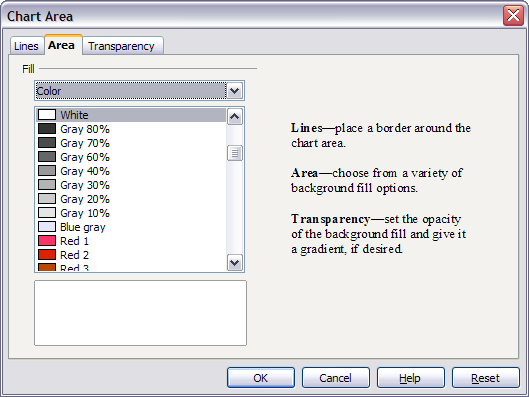
Chart Area dialog.

Changing the chart graphic background

The chart wall is the area that contains the chart graphic.

1. Double-click the chart so that it is enclosed by a gray border.
2. Select Format > Chart Wall. The Chart Wall dialog appears. It has the same formatting options as described in Changing the chart area background.
3. Choose your settings and click OK.

Inserting other objects

Impress offers the capability of inserting in a slide various types of objects such as music or video clips, Writer documents, Math formulas, generic OLE objects and so on. A typical presentation may contain movie clips, sound clips, OLE objects and formulas; other objects are less frequently used since they do not appear during a slide show.

This section covers the part of the Insert menu shown below.

Part of the Insert menu.

Movies and sound

To insert a movie clip or a sound into a presentation, select Insert > Movie and Sound. Select the media file to insert from the dialog, to place the object on the slide.

To insert media clips directly from the Gallery:

1. If not already open, open the Gallery by selecting Tools > Gallery.
2. Browse to the Theme containing media files (for example the Sounds theme).
3. Click on the movie or sound to be inserted and drag it into the slide area.

The Media Playback toolbar is automatically opened; you can preview the media object as well as resize it. If the toolbar does not open, select Tools > Media Player.

The media playback toolbar (movie clip).

The Media Playback toolbar consists of the following elements:

• Add button: opens a dialog where you can select the media file to be inserted.
• Play, Pause, Stop buttons: control the media playback.
• Repeat button: if pressed, the media will restart when finished.
• Playback slider: selects the position within the media clip.
• Timer: displays the current position of the media clip.
• Mute Button: when selected, the sound will be suppressed.
• Volume Slider: adjusts the volume of the media clip.
• Scaling drop-down menu: (only available for movies) allows scaling of the movie clip.

The movie will start playing as soon as the slide is shown during the presentation.

Note that Impress will only link the media clip, therefore when the presentation is moved to a different computer, the link will most likely be broken and as a consequence the media will not play. An easy workaround that prevents this from happening is the following:

1. Place the media file to be included in the presentation in the same folder where the presentation is stored.
2. Insert the media file in the presentation.
3. When sending the presentation to a different computer, send also the media file and place both files in the same folder on the target computer.

Note: At present (OOo 2.1) it is not possible to have a media file played throughout the presentation. It will only be active in the slide where it has been inserted.

Impress offers the possibility to preview the media clips that are to be inserted by means of the provided media player. To open it select Tools > Media Player. The media player is shown in below. Its toolbar is the same as that of the Play Media toolbar described above.

The embedded media player in OpenOffice.org.

OLE objects

Use an OLE (Object Linking and Embedding) object to insert in a presentation either a new document or an existing one. Embedding inserts a copy of the object and details of the source program in the target document, that is the program which is associated to the file type in the operating system. The major benefit of an OLE object is that it is quick and easy to edit the contents just by double-clicking on it. You can also insert a link to the object that will appear as an icon rather than an area showing the contents itself.

To create and insert a new OLE object:

1. Select Insert > Object > OLE object from the main menu. This opens the dialog below.


Insert OLE Object dialog.

2. Select Create new and select the object type among the available options.

Note: “Further objects” is only available under a Windows operating system. It does not appear in the list under any other system.

3. Click OK. An empty container is placed in the slide.
4. Double-click on the OLE object to enter the edit mode of the object. The application devoted to handling that type of file will open the object.

Note: If the object inserted is handled by OpenOffice.org, then the transition to the program to manipulate the object will be seamless; in other cases the object opens in a new window and an option in the File menu becomes available to update the object you inserted.

To insert an existing object:

1. Select Insert > Object > OLE object from the main menu.
2. In the Insert OLE Object dialog, select Create from file. The dialog changes to look like the one below.
3. To insert the object as a link, select the Link to file checkbox. Otherwise, the object will be embedded.
4. Click Search, select the required file in the file picker window, then click Open. A section of the inserted file is shown on the slide.

Inserting an object as a link.

Other OLE objects

Under Windows, the Insert OLE Object dialog has an extra entry, Further objects.

1. Double-click on the entry Further objects to open the dialog shown below.


Advanced menu to insert an OLE object under Windows.

2. Select Create New to insert a new object of the type selected in the Object Type list, or select Create from File to create a new object from a file.
3. If you choose Create from File, the dialog shown below opens. Click Browse and choose the file to insert. The inserted file object is editable by the Windows program that created it. If instead of inserting an object, you want to insert a link to an object, select the Display As Icon checkbox.


Insert object from a file.

Formulas

Use Insert > Object > Formula to create a Math object in a slide. When editing a formula, the main menu changes into the Math main menu.

Care should be taken about the font sizes used in order to make them comparable to the font size used in the rest of the slide. To change the font attributes of the Math object, select Format > Font Size from the main menu bar. To change the font type, select Format > Fonts from the main menu bar.

For additional information on how to create formulas, refer to Chapter 11 (Getting Started with Math) in the Getting Started guide, or Chapter 16 (Math Objects) in the Writer Guide.

Note that unlike in Writer, a formula in Impress is treated as an object, therefore it will not be automatically aligned with the rest of the text. The formula can be however moved around (but not resized) as any other object.

Inserting the contents of a file

You can insert the contents of a file into a presentation. The types of file accepted are OpenOffice.org Draw file, HTML files or plain text files.

Select Insert > File from the main menu to open a file picker window. If there is an internet connection, it is also possible to insert in the file name field a URL. Select the file and click Insert.