Creating formulas
Contents
Introduction
By convention, only three kinds of data can be entered in a cell. Text, Numbers, and Formulas. You can enter formulas in two ways, either in the cell itself, or at the input line. Either way you will need to start it with one of the following symbols: "=", "+" or "-". Starting with anything else will cause the formula to be treated as if it were text.
Operators in formulas
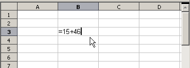
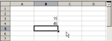
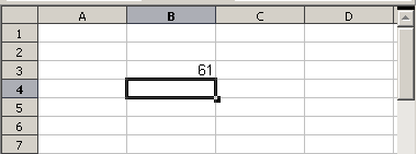
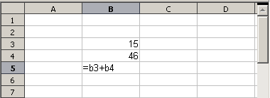
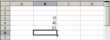
Each cell on the worksheet can be used as a data holder or a place for data calculations. Inserting data is accomplished simply by typing the data in the cell and moving to the next cell or pressing Enter. With formulas the equal sign denotes that instead of the cell being a data holder, the cell will be used for a calculation. A mathematical calculation like 15 + 46 can be accomplished as shown below.
| Simple Calculation in 1 Cell | Calculation by Reference |
|
|
|
|
|
A simple calculation.
While the calculation on the left was accomplished in only one cell, the real power is shown on the right where the data is placed in cells and the calculation is performed using references back to the cells. In this case, cells B3 and B4 were the data holders with B5 the cell where the calculation was performed. Notice that the formula was shown as =B3 + B4. The plus sign denotes addition as the operation being performed upon the data within cells B3 and B4. All formulas build upon this concept. Other ways of entering formulas are shown in Table 1.
These back references to find data to perform a calculation can be found anywhere in the worksheet being worked on or upon any other worksheet in the workbook that is opened. If the data needed was on different worksheets they would be referenced by referring to the worksheet, for example =SUM(Sheet2.B12+Sheet3.A11).
Table 1: Common ways to enter formulas.
| Formula | Description |
|---|---|
| =A1+10 | Displays the contents of cell A1 plus 10. |
| =A1*16% | Displays 16% of the contents of A1. |
| =A1 * A2 | Displays the result of the multiplication of A1 and A2. |
| =ROUND(A1;1) | Displays the contents of cell A1 rounded to one decimal place. |
| =EFFECTIVE(5%;12) | Calculates the effective interest for 5% annual nominal interest with 12 payments a year. |
| =B8-SUM(B10:B14) | Calculates B8 minus the sum of the cells B10 to B14. |
| =SUM(B8;SUM(B10:B14)) | Calculates the sum of cells B10 to B14 and adds the value to B8. |
| =SUM(B1:B65536) | Sums all numbers in column B. |
| =AVERAGE(BloodSugar) | Displays the average of a named range defined under the name BloodSugar. |
| =IF(C31>140; "HIGH"; "OK") | Displays the results of a conditional analysis of data from two sources. If C31 = 144, then HIGH is displayed, otherwise OK is displayed. |
Functions can be identified in Table 1 with a word, for example ROUND, followed by parentheses enclosing references or numbers.
It is also possible to establish ranges for inclusion by naming them using Insert > Names, for example BloodSugar representing a range such as B3:B10. Logical functions can also be performed as represented by the IF statement which results in a conditional response based upon the data in the identified cell.
Operator types
You can use the following operators in OpenOffice.org Calc: arithmetic, comparative, text, and reference.
Arithmetic operators
The addition, subtraction, multiplication and division operators return numerical results. The Negation and Percent operators identify a characteristic of the number found in the cell, for example -37. The example for Exponentiation illustrates how to enter a number that is being multiplied by itself a certain number of times, for example 23 = 2*2*2.
Table 2: Arithmetical operators
| Operator | Name | Example |
| + (Plus) | Addition | =1+1 |
| - (Minus) | Subtraction | =2-1 |
| - (Minus) | Negation | -5 |
| * (asterisk) | Multiplication | =2*2 |
| / (Slash) | Division | =10/5 |
| % (Percent) | Percent | 15% |
| ^ (Caret) | Exponentiation | 2^3 |
Comparative operators
Comparative operators are found in formulas that use the IF function and return either a true or false answer; for example, =IF(B6>G12; 127; 0) which, loosely translated, means if the contents of cell B6 are greater than the contents of cell G12, then return the number 127, otherwise return the number 0.
A direct answer of TRUE or FALSE can be obtained by entering a formula such as =B6>B12. If the numbers found in the referenced cells are accurately represented, the answer TRUE is returned, otherwise FALSE is returned.
Table 3: Comparative operators
| Operator | Name | Example |
| = (equal sign) | Equal | A1=B1 |
| > (Greater than) | Greater than | A1>B1 |
| < (Less than) | Less than | A1<B1 |
| >= (Greater than or equal to) | Greater than or equal to | A1>=B1 |
| <= (Less than or equal to) | Less than or equal to | A1<=B1 |
| <> (Inequality) | Inequality | A1<>B1 |
Text operators
It is common for users to place text in spreadsheets. To provide for variability in what and how this type of data is displayed, text can be joined together in pieces coming from different places on the spreadsheet. Below is an example.
Text Concatenation.
In this example, specific pieces of the text were found in three different cells. To join these segments together, the formula also adds required spaces and punctuation housed within quotation marks resulting in a formula of =B6 & " " & C6 & ", " D6. The result is the concatenation into a correctly formatted date for this locale.
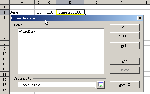
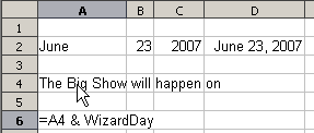
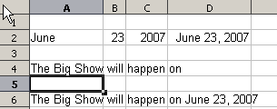
Taking this example further, the result cell is defined as a name, then text concatenation is performed using this defined name.
Defining Names on a worksheet.
Reference operators
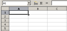
Reference operators merge the values held in each individual cell within the range. Reference operators can be an individual cell identified by the column identifier located along the upper edge of the spreadsheet and a numeric identifier found along the side of the spreadsheet. On spreadsheets read from left to right, the upper left cell is A1. The figure below shows these identifiers for Cell A1.
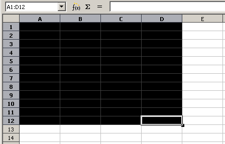
A range is also a reference operator referenced in formulas, functions and logical operators. The range for left to right operations refers to the upper left cell running to the right and downward to the right bottommost cell as shown below.
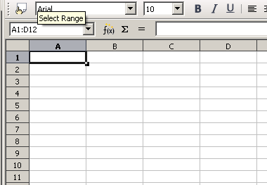
In the upper left corner of the figure above, the range A1:D12 is shown, corresponding to the cells included in the drag operation with the mouse to highlight the range. This same range could also be created by entering in the Name Box directly as shown below. After pressing Enter, the same range is selected.
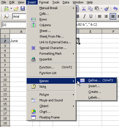
A reference operator can also be created by defining a named area by selecting the menu item Insert > Names > Define, pressing Ctrl+F3, or clicking the icon, if it shows on your toolbar.
Another reference operator involves the use of the '!' sign. If data appears in range A1:B6 as well as range B5:C12, using a formula such as SUM(A1:B6!B5:C12) will yield the sum of cells B5 and B6.
Order of calculation
Order of calculation refers to the sequence that numerical operations are performed. Division and multiplication are performed before addition or subtraction. There is a common tendency to expect calculations to be made from left to right as the equation would be read in English. Calc evaluates the entire formula, then based upon programming precedence breaks the formula down executing multiplication and division operations before other operations. Due to this fact when creating formulas you should test your formula to make sure that the correct result is being obtained. An example of order of calculation in operation follows.
Table 4 – Order of Calculation
| Left To Right Calculation | Ordered Calculation |
| 1+3*2+3 = 11 | =1+3*2+3 result 10 |
| 1+3=4, then 4 X 2 = 8, then 8 + 3 = 11 | 3*2=6, then 1 + 6 + 3 = 10 |
| Another possible intention could be: | The program resolves the multiplication of 3 X 2 before dealing with the numbers being added. |
| 1+3*2+3 = 20 |
If you intend for the result to be either of the two possible solutions on the left, the way to achieve these results would be to order the formula as:
| ((1+3) * 2)+3 = 11 | (1+3) * (2+3) = 20 |
Calculations linking sheets
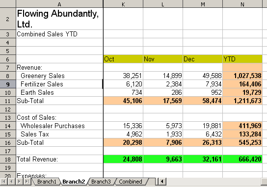
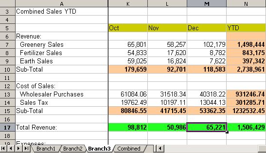
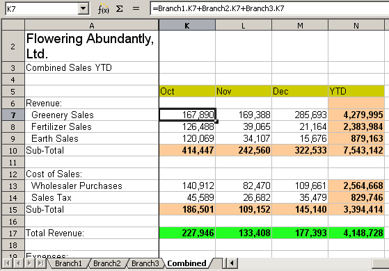
Another powerful feature of Calc is the ability to link data through several worksheets. The naming of worksheets can be helpful to identify where specific data may be found. A name such a Payroll or Boise Sales is much more meaningful than Sheet1. The function named SHEET() returns the sheet number in the collection of spreadsheets. With this function, if you are currently on the third sheet counting from the left along the worksheet tabs, the number 3 is returned. If you drag the worksheets around to different locations among the tabs, the number will return the number referring to the current position of this worksheet.
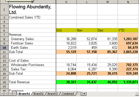
An example of calculations obtaining data from other work can be seen in a business setting where a business combines its branch operations into a single worksheet.
|
Sheet containing data for Branch 1. |
|
Sheet containing data for Branch 2. |
|
Sheet containing data for Branch 3. |
|
Sheet containing combined data for all branches. |
Combining data from several sheets into a single sheet.
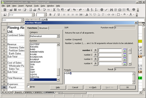
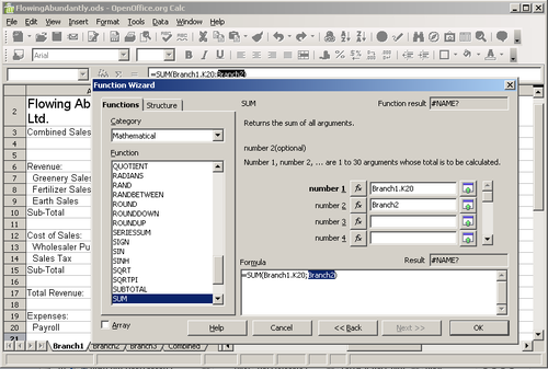
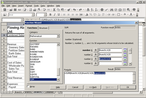
To accomplish the links, it can be easier if the Function Wizard is used.
- Open the Function Wizard by clicking the f(x) button on the toolbar, or by selecting Insert > Function, or by pressing Ctrl+F2.
- Select a category of functions to shorten the list, then scroll down through the named functions and select the required one. When you select a function, its description appears on the right-hand side of the dialog. Double-click on the required function.
- The wizard now displays an area to the right where you can enter data manually in text boxes or click the Shrink button [[Image:]] to shrink the wizard so you can select the cells from the worksheet.
- To select cells, either click directly upon the needed cell or hold down the left mouse button and drag to select the needed area.
- When the area has been selected, click the Shrink button again to return to the wizard.
- If multiple ranges are needed, then select the next text box below the first and perform the same task for the next range. The wizard will accept in the Sum function up to 30 such ranges.
The following figures show how to create the combined sheet shown in the example above.
Strategies for creating formulas
There are several broad approaches when making a decision to create a formula. In deciding on an approach, consider how many other people will need to use the worksheets, the life of the worksheets, and the variations that could be encountered from use.
Enter a unique formula in each cell
The first and most basic strategy is to view whatever formulas are needed as simple and with a limited use life. The strategy is then to place a unique formula in each appropriate cell.
Break formulas into parts and combine the parts
The second strategy is similar, but instead you break down longer formulas into smaller parts and then combine the parts into the whole.
Editor's note: This needs some explanation, but it is NOT about the "formula editor" (Math).
Use the Basic editor to create functions
A third strategy is to use the Basic editor and create your own functions. This approach would be used where the result would greatly simplify the use of the spreadsheet by the end user and keep the formulas simple with a better chance of avoiding errors. This approach also can make the maintenance easier by having corrections or updates kept in one central location. The use of macros is described in Chapter 12 of this book.
| Content on this page is licensed under the Creative Common Attribution 3.0 license (CC-BY). |


